6.4 X11 decomposition

Another popular method for decomposing quarterly and monthly data is the X11 method which originated in the US Census Bureau and Statistics Canada.

This method is based on classical decomposition, but includes many extra steps and features in order to overcome the drawbacks of classical decomposition that were discussed in the previous section. In particular, trend-cycle estimates are available for all observations including the end points, and the seasonal component is allowed to vary slowly over time. X11 also has some sophisticated methods for handling trading day variation, holiday effects and the effects of known predictors. It handles both additive and multiplicative decomposition. The process is entirely automatic and tends to be highly robust to outliers and level shifts in the time series.

The details of the X11 method are described in Dagum and Bianconcini (2016). Here we will only demonstrate how to use the automatic procedure in R.

The X11 method is available using the seas function from the seasonal package for R.

library(seasonal)
elecequip %>% seas(x11="") %>%
autoplot() +
  ggtitle("X11 decomposition of electrical equipment index")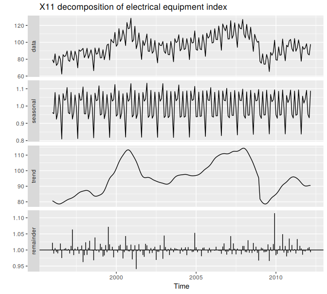

Figure 6.9: An X11 decomposition of the new orders index for electrical equipment.

Compare this decomposition with the STL decomposition shown in Figure 6.1 and the classical decomposition shown in Figure 6.8. The X11 trend-cycle has captured the sudden fall in the data in early 2009 better than either of the other two methods, and the unusual observation at the end of 2009 is now more clearly seen in the remainder component.

Given the output from the seas function, seasonal() will extract the seasonal component, trendcycle() will extract the trend-cycle component, remainder() will extract the remainder component, and seasadj() will compute the seasonally adjusted time series.

For example, Figure 6.10 shows the trend-cycle component and the seasonally adjusted data, along with the original data.

autoplot(elecequip, series="Data") +
  forecast::autolayer(trendcycle(fit), series="Trend") +
  forecast::autolayer(seasadj(fit), series="Seasonally Adjusted") +
  xlab("Year") + ylab("New orders index") +
  ggtitle("Electrical equipment manufacturing (Euro area)") +
  scale_colour_manual(values=c("gray","blue","red"),
                     breaks=c("Data","Seasonally Adjusted","Trend"))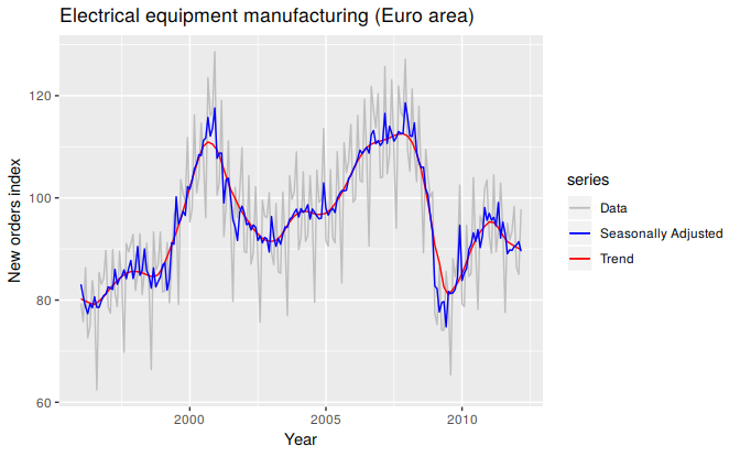

Figure 6.10: Electrical equipment orders: the original data (grey), the trend-cycle component (red) and the seasonally adjusted data (blue).

It can be useful to use seasonal plots and seasonal sub-series plots of the seasonal component. These help us to visualize the variation in the seasonal component over time. Figure 6.11 shows a seasonal sub-series plot of the seasonal component from Figure 6.9. In this case, there are only very small changes over time.

ggsubseriesplot(seasonal(fit)) + ylab("Seasonal")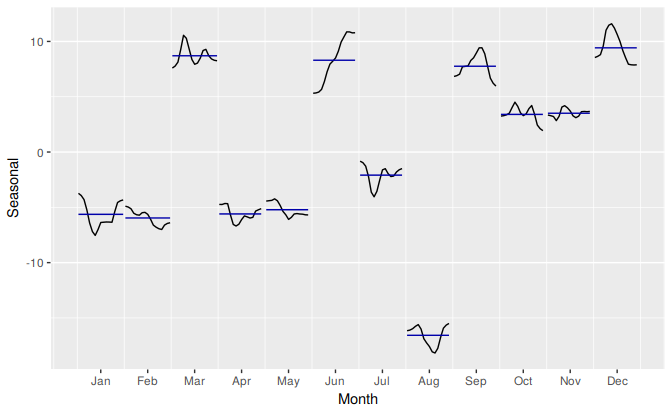

Figure 6.11: Seasonal sub-series plot of the seasonal component from the X11 decomposition shown in Figure 6.9.

References

Dagum, Estela Bee, and Silvia Bianconcini. 2016. Seasonal Adjustment Methods and Real Time Trend-Cycle Estimation: Springer.