5.6 Forecasting with regression

Recall that predictions of \(y\) can be obtained using equation (5.2), \[ \hat{y_t} = \hat\beta_{0} + \hat\beta_{1} x_{1,t} + \hat\beta_{2} x_{2,t} + \cdots + \hat\beta_{k} x_{k,t},\] which comprises the estimated coefficients and ignores the error in the regression equation. Plugging in the values of the predictor variables \(x_{1,t},\ldots,x_{k,t}\) for \(t=1,\ldots,T\) returned the fitted (training-sample) values of \(y\). What we are interested in here is forecasting future values of \(y\).

Ex-ante versus ex-post forecasts

When using regression models for time series data, we need to distinguish between the different types of forecasts that can be produced, depending on what is assumed to be known when the forecasts are computed.

Ex ante forecasts are those that are made using only the information that is available in advance. For example, ex-ante forecasts for the percentage change in US consumption for quarters following the end of the sample, should only use information that was available up to and including 2016 Q3. These are genuine forecasts, made in advance using whatever information is available at the time. Therefore in order to generate ex-ante forecasts, the model requires future values (forecasts) of the predictors. To obtain these we can use one of the simple methods introduced in Section 3.1 or more sophisticated pure time series approaches that follow in Chapters 7 and 8. Alternatively, forecasts from some other source, such as a government agency, may be available and can be used.

Ex post forecasts are those that are made using later information on the predictors. For example, ex post forecasts of consumption may use the actual observations of the predictors, once these have been observed. These are not genuine forecasts, but are useful for studying the behaviour of forecasting models.

The model from which ex-post forecasts are produced should not be estimated using data from the forecast period. That is, ex-post forecasts can assume knowledge of the predictor variables (the \(x\) variables), but should not assume knowledge of the data that are to be forecast (the \(y\) variable).

A comparative evaluation of ex-ante forecasts and ex-post forecasts can help to separate out the sources of forecast uncertainty. This will show whether forecast errors have arisen due to poor forecasts of the predictor or due to a poor forecasting model.

Example: Australian quarterly beer production

Normally, we cannot use actual future values of the predictor variables when producing ex-ante forecasts because their values will not be known in advance. However, the special predictors introduced in Section 5.3 are all known in advance, as they are based on calendar variables (e.g., seasonal dummy variables or public holiday indicators) or deterministic functions of time (e.g. time trend). In such cases, there is no difference between ex ante and ex post forecasts.

beer2 <- window(ausbeer, start=1992)
fit.beer <- tslm(beer2 ~ trend + season)
fcast <- forecast(fit.beer)
autoplot(fcast) +
  ggtitle("Forecasts of beer production using linear regression")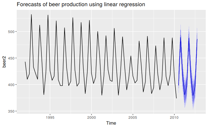

Figure 5.17: Forecasts from the regression model for beer production. The dark shaded region shows 80% prediction intervals and the light shaded region shows 95% prediction intervals.

Scenario based forecasting

In this setting, the forecaster assumes possible scenarios for the predictor variables that are of interest. For example, a US policy maker may be interested in comparing the predicted change in consumption when there is a constant growth of 1% and 0.5% respectively for income and savings with no change in the employment rate, versus a respective decline of 1% and 0.5%, for each of the four quarters following the end of the sample. The resulting forecasts are calculated below and shown in Figure ??. We should note that prediction intervals for scenario based forecasts do not include the uncertainty associated with the future values of the predictor variables. They assume that the values of the predictors are known in advance.

fit.consBest <- tslm(Consumption ~ Income + Savings + Unemployment, data = uschange)
h <- 4
newdata <-
  cbind(Income=c(1,1,1,1), Savings=c(0.5,0.5,0.5,0.5), Unemployment=c(0,0,0,0)) %>%
  as.data.frame()
fcast.up <- forecast(fit.consBest, newdata=newdata)
newdata <-
  cbind(Income=rep(-1,h), Savings=rep(-0.5,h), Unemployment=rep(0,h)) %>%
  as.data.frame()
fcast.down <- forecast(fit.consBest, newdata=newdata)

# autoplot(uschange[,1]) + ylab("% change in US consumption") +
#   forecast::autolayer(fcast.up, PI=TRUE, series="increase") +
#   forecast::autolayer(fcast.down, PI=TRUE, series="decrease") +
#   guides(colour=guide_legend(title="Scenario"))

Building a predictive regression model

The great advantage of regression models is that they can be used to capture important relationships between the forecast variable of interest and the predictor variables. A major challenge however, is that in order to generate ex-ante forecasts the model requires future values of each predictor. If scenario based forecasting is of interest then these models are extremely useful. However, if ex-ante forecasting is the main focus, obtaining forecasts of the predictors can be very challenging (in many cases generating forecasts for the predictor variables can be more challenging than forecasting directly the forecast variable without using predictors).

An alternative formulation is to use as predictors their lagged values. Assuming that we are interested in generating a \(h\)-step ahead forecast we write \[y_{t+h}=\beta_0+\beta_1x_{1,t}+\dots+\beta_kx_{k,t}+\varepsilon_{t+h}\] for \(h=1,2\ldots\). The predictor set is formed by values of the \(x\)s that are observed \(h\) time periods prior to observing \(y\). Therefore when the estimated model is projected into the future, i.e., beyond the end of the sample \(T\), all predictor values are available.

Including lagged values of the predictors does not only make the model operational for easily generating forecasts, it also makes it intuitively appealling. For example, the effect of a policy change with the aim of increasing production may not have an instantaneous effect on consumption expenditure. It is most likely that this will happend with a lagging effect. We touched upon this in Section 5.3 when briefly introducing distributed lags as predictors. Several directions for generalising regression models to better incorporate the rich dynamics observed in time series are discussed In Section 9.

Prediction intervals

With each forecast for the change in consumption Figure ?? 95% and 80% prediction intervals are also included. The general formulation of how to calculate prediction intervals for multiple regression models is presented in Section 5.7. As this involves some advanced matrix algebra we present here the case for calculating prediction intervals for a simple regression, where a forecast can be generated using the equation, \[\hat{y}=\hat{\beta}_0+\hat{\beta}_1x.\] Assuming that the regression errors are normally distributed, an approximate 95% prediction interval (also called a prediction interval) associated with this forecast is given by \[\begin{equation} \hat{y} \pm 1.96 \hat{\sigma}_e\sqrt{1+\frac{1}{T}+\frac{(x-\bar{x})^2}{(T-1)s_x^2}}, \tag{5.4} \end{equation}\] where \(T\) is the total number of observations, \(\bar{x}\) is the mean of the observed \(x\) values, \(s_x\) is the standard deviation of the observed \(x\) values and \(\hat{\sigma}_e\) is the standard error of the regression given by Equation (5.3). Similarly, an 80% prediction interval can be obtained by replacing 1.96 by 1.28. Other prediction intervals can be obtained by replacing the 1.96 with the appropriate value given in Table 3.1. If R is used to obtain prediction intervals, more exact calculations are obtained (especially for small values of \(T\)) than what is given by Equation (5.4).

Equation (5.4) shows that the prediction interval is wider when \(x\) is far from \(\bar{x}\). That is, we are more certain about our forecasts when considering values of the predictor variable close to its sample mean. #### Example {-} TODO: This is to higligh the extreme case. If not useful just remove.

The estimated simple regression line in the US consumption example is \[ \hat{y}_t=0.55 + 0.28x_t. \]

Assuming that for the next four quarters personal income will increase by its historical mean value of \(\bar{x}=0.72\%\), consumption is forecast to increase by \(0.75\%\) and the corresponding \(95\%\) and \(80\%\) prediction intervals are \([-0.45,1.94]\) and \([-0.03,1.52]\) respectively (calcualted using R). If we assume an extreme increase of \(10\%\) in income then the prediction intervals are considerably wider as shown in Figure ??.

# autoplot(uschange[,"Consumption"]) +
#   ylab("% change in US consumption") +
#   forecast::autolayer(fcast.up, PI=TRUE, series="Average increase") +
#   forecast::autolayer(fcast.down, PI=TRUE, series="Extreme increase") +
#   guides(colour=guide_legend(title="Scenario"))