2.9 White noise

Time series that show no autocorrelation are called “white noise”. Figure 2.13 gives an example of a white noise series.

set.seed(30)
y <- ts(rnorm(50))
autoplot(y) + ggtitle("White noise")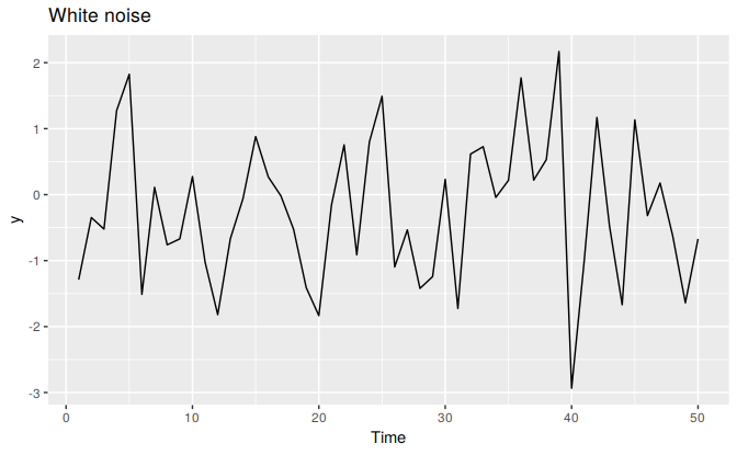

Figure 2.13: A white noise time series.

ggAcf(y)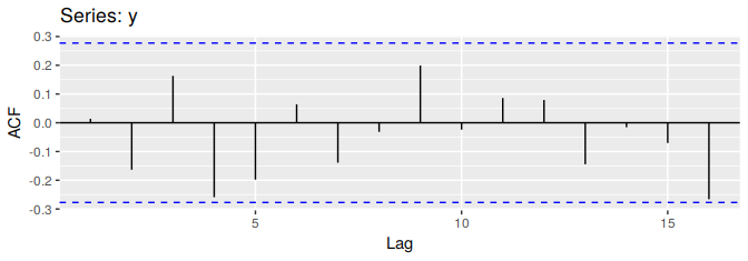

Figure 2.14: Autocorrelation function for the white noise series.

For white noise series, we expect each autocorrelation to be close to zero. Of course, they will not be exactly equal to zero as there is some random variation. For a white noise series, we expect 95% of the spikes in the ACF to lie within \(\pm 2/\sqrt{T}\) where \(T\) is the length of the time series. It is common to plot these bounds on a graph of the ACF (the blue dashed lines above). If one or more large spikes are outside these bounds, or if substantially more than 5% of spikes are outside these bounds, then the series is probably not white noise.

In this example, \(T=50\) and so the bounds are at \(\pm 2/\sqrt{50} = \pm 0.28\). All of the autocorrelation coefficients lie within these limits, confirming that the data are white noise.