• Forecasting: Principles and Practice
  • Welcome
  • 1 Getting started
    • 1.1 What can be forecast?
    • 1.2 Forecasting, planning and goals
    • 1.3 Determining what to forecast
    • 1.4 Forecasting data and methods
    • 1.5 Some case studies
    • 1.6 The basic steps in a forecasting task
    • 1.7 The statistical forecasting perspective
    • 1.8 Exercises
    • 1.9 Further reading
  • 2 Time series graphics
    • 2.1 ts objects
    • 2.2 Time plots
    • 2.3 Time series patterns
    • 2.4 Seasonal plots
    • 2.5 Seasonal subseries plots
    • 2.6 Scatterplots
    • 2.7 Lag plots
    • 2.8 Autocorrelation
    • 2.9 White noise
    • 2.10 Exercises
    • 2.11 Further reading
  • 3 The forecaster’s toolbox
    • 3.1 Some simple forecasting methods
    • 3.2 Transformations and adjustments
    • 3.3 Residual diagnostics
    • 3.4 Evaluating forecast accuracy
    • 3.5 Prediction intervals
    • 3.6 The forecast package in R
    • 3.7 Exercises
    • 3.8 Further reading
  • 4 Judgmental forecasts
    • 4.1 Beware of limitations
    • 4.2 Key principles
    • 4.3 The Delphi method
    • 4.4 Forecasting by analogy
    • 4.5 Scenario Forecasting
    • 4.6 New product forecasting
    • 4.7 Judgmental adjustments
    • 4.8 Further reading
  • 5 Linear regression models
    • 5.1 The linear model
    • 5.2 Least squares estimation
    • 5.3 Some useful predictors
    • 5.4 Evaluating the regression model
    • 5.5 Selecting predictors
    • 5.6 Forecasting with regression
    • 5.7 Matrix formulation
    • 5.8 Nonlinear regression
    • 5.9 Correlation, causation and forecasting
    • 5.10 Exercises
    • 5.11 Further reading
  • 6 Time series decomposition
    • 6.1 Time series components
    • 6.2 Moving averages
    • 6.3 Classical decomposition
    • 6.4 X11 decomposition
    • 6.5 SEATS decomposition
    • 6.6 STL decomposition
    • 6.7 Forecasting with decomposition
    • 6.8 Exercises
    • 6.9 Further reading
  • 7 Exponential smoothing
    • 7.1 Simple exponential smoothing
    • 7.2 Trend methods
    • 7.3 Holt-Winters’ seasonal method
    • 7.4 A taxonomy of exponential smoothing methods
    • 7.5 Innovations state space models for exponential smoothing
    • 7.6 Estimation and model selection
    • 7.7 Forecasting with ETS models
    • 7.8 Exercises
    • 7.9 Further reading
  • 8 ARIMA models
    • 8.1 Stationarity and differencing
    • 8.2 Backshift notation
    • 8.3 Autoregressive models
    • 8.4 Moving average models
    • 8.5 Non-seasonal ARIMA models
    • 8.6 Estimation and order selection
    • 8.7 ARIMA modelling in R
    • 8.8 Forecasting
    • 8.9 Seasonal ARIMA models
    • 8.10 ARIMA vs ETS
    • 8.11 Exercises
  • 9 Dynamic regression models
    • 9.1 Estimation
    • 9.2 Regression with ARIMA errors in R
    • 9.3 Forecasting
    • 9.4 Stochastic and deterministic trends
    • 9.5 Dynamic harmonic regression
    • 9.6 Lagged predictors
    • 9.7 Exercises
    • 9.8 Further reading
  • 10 Forecasting hierarchical or grouped time series
    • 10.1 Hierarchical time series
    • 10.2 Grouped time series
    • 10.3 Base and coherent forecasts
    • 10.4 The bottom-up approach
    • 10.5 Top-down approaches
    • 10.6 Middle-out approach
    • 10.7 The projection matrix
    • 10.8 The optimal reconciliation approach
    • 10.9 Exercises
    • 10.10 Further reading
  • 11 Advanced forecasting methods
    • 11.1 Complex seasonality
    • 11.2 Forecasting counts
    • 11.3 Vector autoregressions
    • 11.4 Neural network models
    • 11.5 Exercises
  • 12 Some practical forecasting issues
    • 12.1 Weekly, daily and sub-daily data
    • 12.2 Time series of counts
    • 12.3 Ensuring forecasts stay within limits
    • 12.4 Forecast combinations
    • 12.5 Prediction intervals for aggregates
    • 12.6 Backcasting
    • 12.7 Forecasting very short time series
    • 12.8 Forecasting very long time series
    • 12.9 One-step forecasts on test data
    • 12.10 Multi-step forecasts on training data
    • 12.11 Dealing with missing values and outliers
    • 12.12 Bootstrapping and bagging
  • Using R
  • References
  • Published by OTexts with bookdown

Forecasting: Principles and Practice

9.4 Stochastic and deterministic trends

There are two different ways of modelling a linear trend. A deterministic trend is obtained using the regression model \[ y_t = \beta_0 + \beta_1 t + n_t, \] where \(n_t\) is an ARMA process. A stochastic trend is obtained using the model \[ y_t = \beta_0 + \beta_1 t + n_t, \] where \(n_t\) is an ARIMA process with \(d=1\). In that case, we can difference both sides so that \(y_t' = \beta_1 + n_t'\), where \(n_t'\) is an ARMA process. In other words, \[ y_t = y_{t-1} + \beta_1 + n_t'. \] This is very similar to a random walk with drift, but here the error term is an ARMA process rather than simply white noise.

Although these models appear quite similar (they only differ in the number of differences that need to be applied to \(n_t\)), their forecasting characteristics are quite different.

Example: International visitors to Australia

autoplot(austa) + xlab("Year") +
  ylab("millions of people") +
  ggtitle("Total annual international visitors to Australia")
Annual international visitors to Australia, 1980--2010.

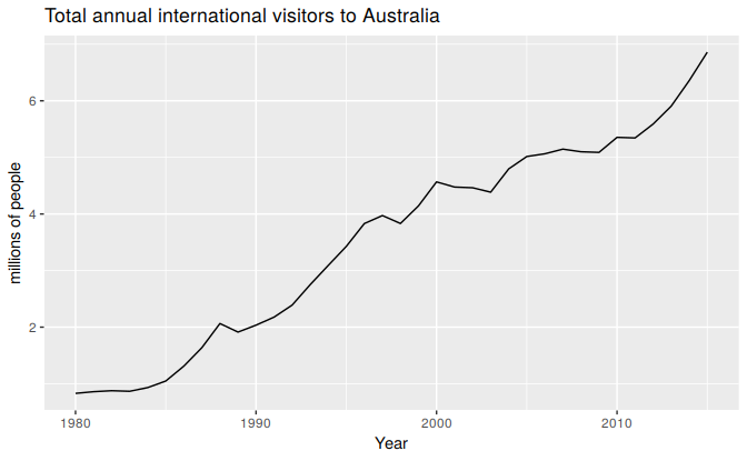
Figure 9.7: Annual international visitors to Australia, 1980–2010.

Figure 9.7 shows the total number of international visitors to Australia each year from 1980 to 2010. We will fit both a deterministic and a stochastic trend model to these data.

The deterministic trend model is obtained as follows:

trend <- seq_along(austa)
(fit1 <- auto.arima(austa, d=0, xreg=trend))
#> Series: austa 
#> Regression with ARIMA(2,0,0) errors 
#> 
#> Coefficients:
#>        ar1     ar2  intercept   xreg
#>       1.11  -0.380      0.416  0.171
#> s.e.  0.16   0.158      0.190  0.009
#> 
#> sigma^2 estimated as 0.0298:  log likelihood=13.6
#> AIC=-17.2   AICc=-15.2   BIC=-9.28

This model can be written as \[\begin{align*} y_t &= 0.42 + 0.17 t + n_t \\ n_t &= 1.11 n_{t-1} -0.38 n_{t-2} + e_t\\ e_t &\sim \text{NID}(0,0.0298). \end{align*}\]

The estimated growth in visitor numbers is 0.17 million people per year.

Alternatively, the stochastic trend model can be estimated.

(fit2 <- auto.arima(austa, d=1))
#> Series: austa 
#> ARIMA(0,1,1) with drift 
#> 
#> Coefficients:
#>         ma1  drift
#>       0.301  0.173
#> s.e.  0.165  0.039
#> 
#> sigma^2 estimated as 0.0338:  log likelihood=10.6
#> AIC=-15.2   AICc=-14.5   BIC=-10.6

This model can be written as \(y_t-y_{t-1} = 0.17 + n'_t\), or equivalently \[\begin{align*} y_t &= y_0 + 0.17 t + n_t \\ n_t &= n_{t-1} + 0.30 e_{t-1} + e_{t}\\ e_t &\sim \text{NID}(0,0.0338). \end{align*}\]

In this case, the estimated growth in visitor numbers is also 0.17 million people per year. Although the growth estimates are similar, the prediction intervals are not, as Figure ?? shows. In particular, stochastic trends have much wider prediction intervals because the errors are non-stationary.

# fc1 <- forecast(fit1, xreg=data.frame(trend=length(austa)+1:10))
# fc2 <- forecast(fit2, h=10)
# autoplot(austa) +
#   forecast::autolayer(fc2, series="Stochastic trend") +
#   forecast::autolayer(fc1, series="Deterministic trend") +
#   ggtitle("Forecasts from deterministic and stochastic trend models") +
#   xlab("Year") + ylab("Visitors to Australia (millions)") +
#   guides(colour=guide_legend(title="Forecast"))

There is an implicit assumption with deterministic trends that the slope of the trend is not going to change over time. On the other hand, stochastic trends can change, and the estimated growth is only assumed to be the average growth over the historical period, not necessarily the rate of growth that will be observed into the future. Consequently, it is safer to forecast with stochastic trends, especially for longer forecast horizons, as the prediction intervals allow for greater uncertainty in future growth.