3.3 Residual diagnostics
Fitted values
Each observation in a time series can be forecast using all previous observations. We call these “fitted values” and they are denoted by \(\hat{y}_{t|t-1}\), meaning the forecast of \(y_t\) based on observations \(y_{1},\dots,y_{t-1}\) . We use these so often, we sometimes drop part of the subscript and just write \(\hat{y}_t\) instead of \(\hat{y}_{t|t-1}\). Fitted values always involve one-step forecasts.
Actually, fitted values are often not true forecasts because any parameters involved in the forecasting method are estimated using all available observations in the time series, including future observations. For example, if we use the average method, the fitted values are given by \[ \hat{y}_t = \hat{c} \] where \(\hat{c}\) is the average computed over all available observations, including those at times after \(t\). Similarly, for the drift method, the drift parameter is estimated using all available observations. In this case, the fitted values are given by \[ \hat{y}_t = y_{t-1} + \hat{c} \] where \[ \hat{c} = (y_T-y_1)/(T-1). \] In both cases, there is a parameter to be estimated from the data. The “hat” above the \(c\) reminds us that this is an estimate. When the estimate of \(c\) involves observations after time \(t\), the fitted values are not true forecasts. On the other hand, naïve or seasonal naïve forecasts do not involve any parameters, and so fitted values are true forecasts in such cases.
Residuals
The “residuals” in a time series model are what is left over after fitting a model. For many (but not all) time series models, the residuals are equal to the difference between the observations and the corresponding fitted values: \[ e_{t} = y_{t}-\hat{y}_{t}. \]
Residuals are useful in checking whether a model has adequately captured the information in the data. A good forecasting method will yield residuals with the following properties:
- The residuals are uncorrelated. If there are correlations between residuals, then there is information left in the residuals which should be used in computing forecasts.
- The residuals have zero mean. If the residuals have a mean other than zero, then the forecasts are biased.
Any forecasting method that does not satisfy these properties can be improved. However, that does not mean that forecasting methods that satisfy these properties cannot be improved. It is possible to have several different forecasting methods for the same data set, all of which satisfy these properties. Checking these properties is important in order to see whether a method is using all of the available information, but it is not a good way to select a forecasting method.
If either of these properties is not satisfied, then the forecasting method can be modified to give better forecasts. Adjusting for bias is easy: if the residuals have mean \(m\), then simply add \(m\) to all forecasts and the bias problem is solved. Fixing the correlation problem is harder, and we will not address it until Chapter 9.
In addition to these essential properties, it is useful (but not necessary) for the residuals to also have the following two properties.
- The residuals have constant variance.
- The residuals are normally distributed.
These two properties make the calculation of prediction intervals easier (see Section 3.5 for an example). However, a forecasting method that does not satisfy these properties cannot necessarily be improved. Sometimes applying a Box-Cox transformation may assist with these properties, but otherwise there is usually little that you can do to ensure that your residuals have constant variance and a normal distribution. Instead, an alternative approach to obtaining prediction intervals is necessary. Again, we will not address how to do this until later in the book.
Example: Forecasting the Dow-Jones Index
For stock market indexes, the best forecasting method is often the naïve method. That is, each forecast is simply equal to the last observed value, or \(\hat{y}_{t} = y_{t-1}\). Hence, the residuals are simply equal to the difference between consecutive observations: \[ e_{t} = y_{t} - \hat{y}_{t} = y_{t} - y_{t-1}. \]
The following graphs show the Dow Jones Index (DJI), and the residuals obtained from forecasting the DJI using the naïve method.
dj2 <- window(dj, end=250)
autoplot(dj2) + xlab("Day") + ylab("") +
  ggtitle("Dow Jones Index (daily ending 15 Jul 94)")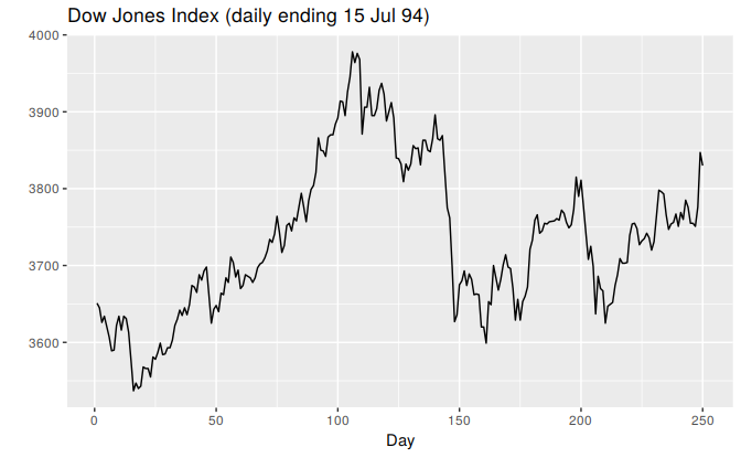
Figure 3.4: The Dow Jones Index measured daily to 15 July 1994.
res <- residuals(naive(dj2))
autoplot(res) + xlab("Day") + ylab("") +
  ggtitle("Residuals from naïve method")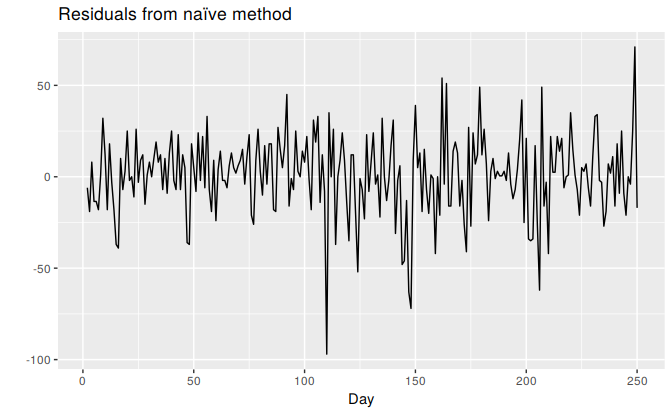
Figure 3.5: Residuals from forecasting the Dow Jones Index using the naïve method.
gghistogram(res) + ggtitle("Histogram of residuals")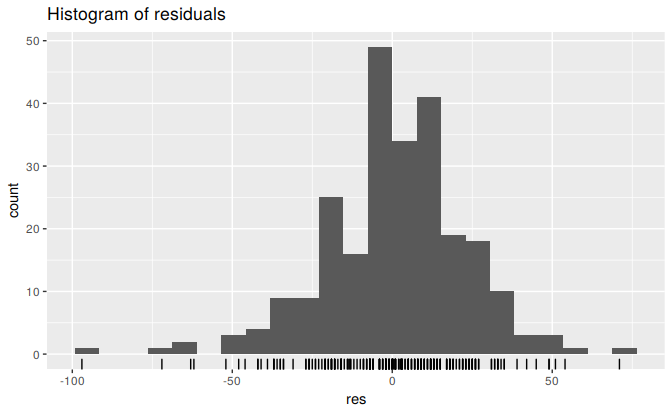
Figure 3.6: Histogram of the residuals from the naïve method applied to the Dow Jones Index. The left tail is a little too long for a normal distribution.
ggAcf(res) + ggtitle("ACF of residuals")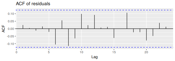
Figure 3.7: ACF of the residuals from the naïve method applied to the Dow Jones Index. The lack of correlation suggesting the forecasts are good.
These graphs show that the naïve method produces forecasts that appear to account for all available information. The mean of the residuals is very close to zero and there is no significant correlation in the residuals series. The time plot of the residuals shows that the variation of the residuals stays much the same across the historical data, so the residual variance can be treated as constant. However, the histogram suggests that the residuals may not follow a normal distribution — the left tail looks a little too long. Consequently, forecasts from this method will probably be quite good, but prediction intervals that are computed assuming a normal distribution may be inaccurate.
Portmanteau tests for autocorrelation
In addition to looking at the ACF plot, we can also do a more formal test for autocorrelation by considering a whole set of \(r_k\) values as a group, rather than treating each one separately.
Recall that \(r_k\) is the autocorrelation for lag \(k\). When we look at the ACF plot to see whether each spike is within the required limits, we are implicitly carrying out multiple hypothesis tests, each one with a small probability of giving a false positive. When enough of these tests are done, it is likely that at least one will give a false positive, and so we may conclude that the residuals have some remaining autocorrelation, when in fact they do not.
In order to overcome this problem, we test whether the first \(h\) autocorrelations are significantly different from what would be expected from a white noise process. A test for a group of autocorrelations is called a portmanteau test, from a French word describing a suitcase containing a number of items.
One such test is the Box-Pierce test, based on the following statistic \[ Q = T \sum_{k=1}^h r_k^2, \] where \(h\) is the maximum lag being considered and \(T\) is the number of observations. If each \(r_k\) is close to zero, then \(Q\) will be small. If some \(r_k\) values are large (positive or negative), then \(Q\) will be large. We suggest using \(h=10\) for non-seasonal data and \(h=2m\) for seasonal data, where \(m\) is the period of seasonality. However, the test is not good when \(h\) is large, so if these values are larger than \(T/5\), then use \(h=T/5\)
A related (and more accurate) test is the Ljung-Box test, based on \[ Q^* = T(T+2) \sum_{k=1}^h (T-k)^{-1}r_k^2. \]
Again, large values of \(Q^*\) suggest that the autocorrelations do not come from a white noise series.
How large is too large? If the autocorrelations did come from a white noise series, then both \(Q\) and \(Q^*\) would have a \(\chi^2\) distribution with \((h - K)\) degrees of freedom, where \(K\) is the number of parameters in the model. If they are calculated from raw data (rather than the residuals from a model), then set \(K=0\).
For the Dow-Jones example, the naïve model has no parameters, so \(K=0\) in that case also.
# lag=h and fitdf=K
Box.test(res, lag=10, fitdf=0)
#>
#>  Box-Pierce test
#>
#> data:  res
#> X-squared = 11, df = 10, p-value = 0.4

Box.test(res,lag=10, fitdf=0, type="Lj")
#>
#>  Box-Ljung test
#>
#> data:  res
#> X-squared = 11, df = 10, p-value = 0.4
For both \(Q\) and \(Q^*\), the results are not significant (i.e., the \(p\)-values are relatively large). Thus, we can conclude that the residuals are not distinguishable from a white noise series.
All of these methods for checking residuals are conveniently packaged into one R function, which will produce a time plot, ACF plot and histogram of the residuals (with an overlayed normal distribution for comparison), and do a Ljung-Box test with the correct degrees of freedom:
checkresiduals(naive(dj2))
#>
#>  Ljung-Box test
#>
#> data:  Residuals from Naive method
#> Q* = 11, df = 10, p-value = 0.4
#>
#> Model df: 0.   Total lags used: 10