9.3 Forecasting

To forecast a regression model with ARIMA errors, we need to forecast the regression part of the model and the ARIMA part of the model, and combine the results. As with ordinary regression models, in order to obtain forecasts we first need to forecast the predictors. When the predictors are known into the future (e.g., calendar-related variables such as time, day-of-week, etc.), this is straightforward. But when the predictors are themselves unknown, we must either model them separately, or use assumed future values for each predictor.

Example: US Personal Consumption and Income

We will calculate forecasts for the next eight quarters assuming that the future percentage changes in personal disposable income will be equal to the mean percentage change from the last forty years.

fcast <- forecast(fit, xreg=rep(mean(uschange[,2]),8))
autoplot(fcast) + xlab("Year") +
  ylab("Percentage change")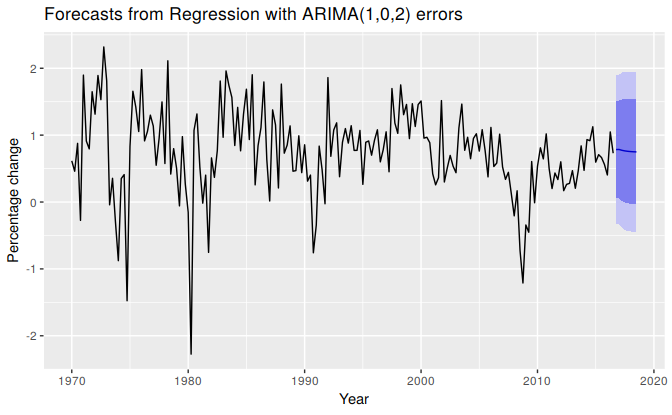

Figure 9.4: Forecasts obtained from regressing the percentage change in consumption expenditure on the percentage change in disposable income, with an ARIMA(1,0,2) error model.

The prediction intervals for this model are narrower than those for the model developed in Section 8.5 because we are now able to explain some of the variation in the data using the income predictor.

It is important to realise that the prediction intervals from regression models (with or without ARIMA errors) do not take into account the uncertainty in the forecasts of the predictors. So they should be interpreted as being conditional on the assumed (or estimated) future values of the predictor variables.

Example: Forecasting electricity demand

Daily electricity demand can be modelled as a function of temperature. As can be observed on an electricity bill, more electricity is used on cold days due to heating and hot days due to air conditioning. The higher demand on cold and hot days is reflected in the u-shape of Figure 9.5, where daily demand is plotted versus daily maximum temperature.

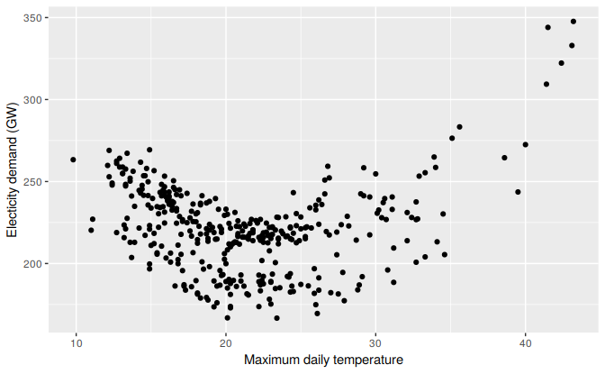
Figure 9.5: Daily electricity demand versus maximum daily temperature for the state of Victoria in Australia for 2014.

The data are stored as elecdaily including total daily demand, an indicator variable for workdays (a workday is represented with 1, and a non-workday is represented with 0), and daily maximum temperatures. Because there is weekly seasonality, the frequency has been set to 7. Figure 9.6 show the time series of both daily demand and daily maximum temperatures. The plots highlight the need for both a non-linear and also dynamic model.

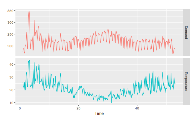
Figure 9.6: Daily electricity demand and maximum daily temperature for the state of Victoria in Australia for 2014.

In this example, we fit a quadratic regression model with ARMA errors using the auto.arima function. Using the estimated model we forecast 14 days ahead starting from Thursday 1 January 2015 (a non-work-day being a public holiday for New Years Day).

In this case, we could obtain weather forecasts from the weather bureau for the next 14 days. But for the sake of illustration, we will use scenario based forecasting (as introduced in Section 5.6) where we set the temperature for the next 14 days to a constant 26 degrees.

xreg <- cbind(MaxTemp = elecdaily[, "Temperature"], 
              MaxTempSq = elecdaily[, "Temperature"]^2, 
              Workday = elecdaily[, "WorkDay"])
fit <- auto.arima(elecdaily[, "Demand"], xreg = xreg)
checkresiduals(fit)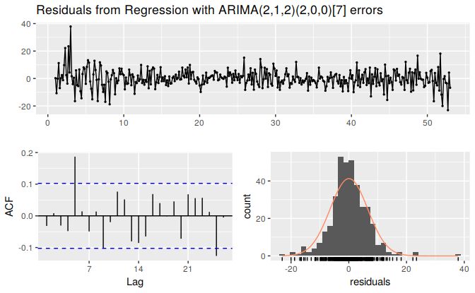

#> 
#>  Ljung-Box test
#> 
#> data:  Residuals from Regression with ARIMA(2,1,2)(2,0,0)[7] errors
#> Q* = 28, df = 4, p-value = 1e-05
#> 
#> Model df: 10.   Total lags used: 14

The model has some significant autocorrelation in the residuals, which means the prediction intervals may not provide accurate coverage. Also, the histogram of the residuals shows one positive outlier, which will also affect the coverage of the prediction intervals.

autoplot(elecdaily[,'Demand'], series="Data") +
  forecast::autolayer(fitted(fit), series="Fitted") +
  ylab("") +
  ggtitle("Daily electricity demand (GW)") +
  guides(colour=guide_legend(title=" "))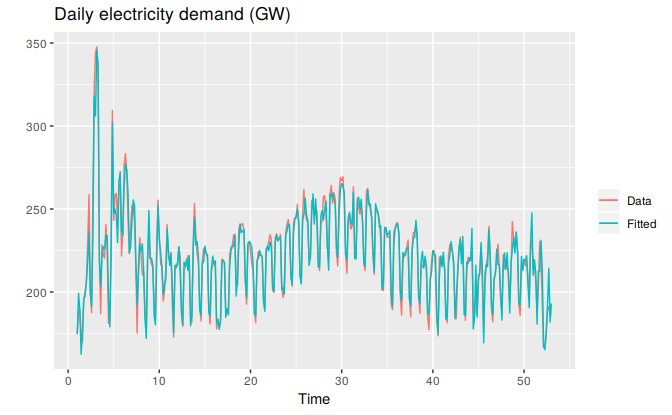

fcast <- forecast(fit, 
  xreg = cbind(rep(26,14), rep(26^2,14), c(0,1,0,0,1,1,1,1,1,0,0,1,1,1)))
#> Warning in forecast.Arima(fit, xreg = cbind(rep(26, 14), rep(26^2, 14), :
#> xreg contains different column names from the xreg used in training. Please
#> check that the regressors are in the same order.
autoplot(fcast) + ylab("Electicity demand (GW)")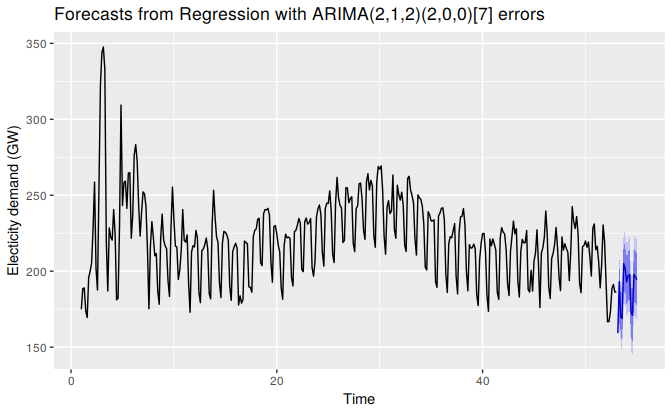 

The point forecasts look reasonable for the first two weeks of 2015. The slow down in electricity demand at the end of 2014 has caused the forecasts for the next two weeks to show similarly low demand values.