8.9 Seasonal ARIMA models

So far, we have restricted our attention to non-seasonal data and non-seasonal ARIMA models. However, ARIMA models are also capable of modelling a wide range of seasonal data.

A seasonal ARIMA model is formed by including additional seasonal terms in the ARIMA models we have seen so far. It is written as follows:

ARIMA	$~\underbrace{(p, d, q)}$	$\underbrace{(P, D, Q)_{m}}$
	${\uparrow}$	${\uparrow}$
	Non-seasonal part	Seasonal part of
	of the model	of the model

where $m =$ number of observations per year. We use uppercase notation for the seasonal parts of the model, and lowercase notation for the non-seasonal parts of the model.

The seasonal part of the model consists of terms that are very similar to the non-seasonal components of the model, but involve backshifts of the seasonal period. For example, an ARIMA(1,1,1)(1,1,1)$_{4}$ model (without a constant) is for quarterly data ($m=4$), and can be written as \[ (1 - \phi_{1}B)~(1 - \Phi_{1}B^{4}) (1 - B) (1 - B^{4})y_{t} = (1 + \theta_{1}B)~ (1 + \Theta_{1}B^{4})e_{t}. \]

The additional seasonal terms are simply multiplied by the non-seasonal terms.

ACF/PACF

The seasonal part of an AR or MA model will be seen in the seasonal lags of the PACF and ACF. For example, an ARIMA(0,0,0)(0,0,1)$_{12}$ model will show:

a spike at lag 12 in the ACF but no other significant spikes;
exponential decay in the seasonal lags of the PACF (i.e., at lags 12, 24, 36, …).

Similarly, an ARIMA(0,0,0)(1,0,0)$_{12}$ model will show:

exponential decay in the seasonal lags of the ACF;
a single significant spike at lag 12 in the PACF.

In considering the appropriate seasonal orders for an ARIMA model, restrict attention to the seasonal lags.

The modelling procedure is almost the same as for non-seasonal data, except that we need to select seasonal AR and MA terms as well as the non-seasonal components of the model. The process is best illustrated via examples.

Example: European quarterly retail trade

We will describe the seasonal ARIMA modelling procedure using quarterly European retail trade data from 1996 to 2011. The data are plotted in Figure 8.15.

autoplot(euretail) + ylab("Retail index") + xlab("Year")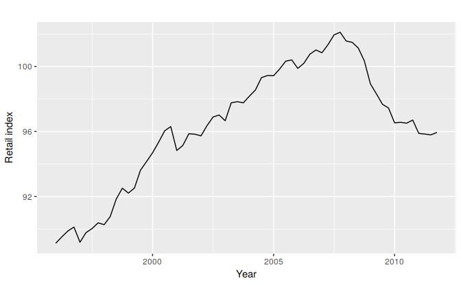

Quarterly retail trade index in the Euro area (17 countries), 1996--2011, covering wholesale and retail trade, and the repair of motor vehicles and motorcycles. (Index: 2005 = 100).

Figure 8.15: Quarterly retail trade index in the Euro area (17 countries), 1996–2011, covering wholesale and retail trade, and the repair of motor vehicles and motorcycles. (Index: 2005 = 100).

The data are clearly non-stationary, with some seasonality, so we will first take a seasonal difference. The seasonally differenced data are shown in Figure 8.16. These also appear to be non-stationary, so we take an additional first difference, shown in Figure 8.17.

euretail %>% diff(lag=4) %>% ggtsdisplay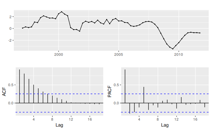

Figure 8.16: Seasonally differenced European retail trade index.

euretail %>% diff(lag=4) %>% diff() %>% ggtsdisplay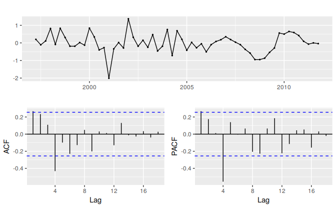

Figure 8.17: Double differenced European retail trade index.

Our aim now is to find an appropriate ARIMA model based on the ACF and PACF shown in Figure 8.17. The significant spike at lag 1 in the ACF suggests a non-seasonal MA(1) component, and the significant spike at lag 4 in the ACF suggests a seasonal MA(1) component. Consequently, we begin with an ARIMA(0,1,1)(0,1,1)$_4$ model, indicating a first and seasonal difference, and non-seasonal and seasonal MA(1) components. The residuals for the fitted model are shown in Figure 8.18. (By analogous logic applied to the PACF, we could also have started with an ARIMA(1,1,0)(1,1,0)$_4$ model.)

euretail %>%
  Arima(order=c(0,1,1), seasonal=c(0,1,1)) %>%
  residuals %>%
  ggtsdisplay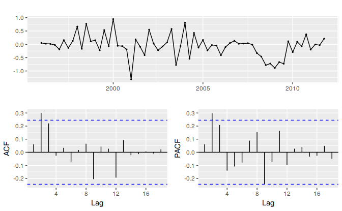

Figure 8.18: Residuals from the fitted ARIMA(0,1,3)(0,1,1)$_4$ model for the European retail trade index data.

Both the ACF and PACF show significant spikes at lag 2, and almost significant spikes at lag 3, indicating that some additional non-seasonal terms need to be included in the model. The AICc of the ARIMA(0,1,2)(0,1,1)$_4$ model is 74.36, while that for the ARIMA(0,1,3)(0,1,1)$_4$ model is 68.53. We tried other models with AR terms as well, but none that gave a smaller AICc value. Consequently, we choose the ARIMA(0,1,3)(0,1,1)$_4$ model. Its residuals are plotted in Figure 8.19. All the spikes are now within the significance limits, so the residuals appear to be white noise. The Ljung-Box test also shows that the residuals have no remaining autocorrelations.

fit3 <- Arima(euretail, order=c(0,1,3), seasonal=c(0,1,1))
checkresiduals(fit3)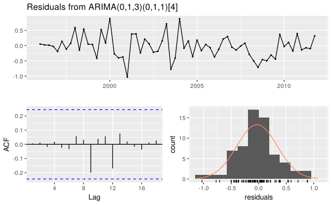

Figure 8.19: Residuals from the fitted ARIMA(0,1,3)(0,1,1)$_4$ model for the European retail trade index data.

#> 
#>  Ljung-Box test
#> 
#> data:  Residuals from ARIMA(0,1,3)(0,1,1)[4]
#> Q* = 0.5, df = 4, p-value = 1
#> 
#> Model df: 4.   Total lags used: 8

Thus, we now have a seasonal ARIMA model that passes the required checks and is ready for forecasting. Forecasts from the model for the next three years are shown in Figure 8.20. The forecasts follow the recent trend in the data, because of the double differencing. The large and rapidly increasing prediction intervals show that the retail trade index could start increasing or decreasing at any time — while the point forecasts trend downwards, the prediction intervals allow for the data to trend upwards during the forecast period.

fit3 %>% forecast(h=12) %>% autoplot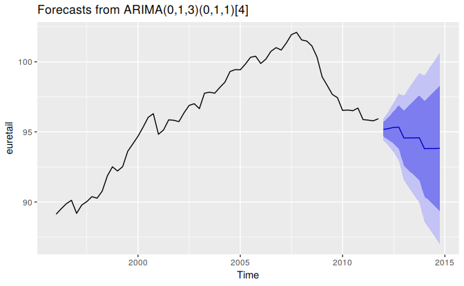

Figure 8.20: Forecasts of the European retail trade index data using the ARIMA(0,1,3)(0,1,1)$_4$ model. 80% and 95% prediction intervals are shown.

We could have used auto.arima() to do most of this work for us. It would have given the following result.

auto.arima(euretail)
#> Series: euretail 
#> ARIMA(0,1,3)(0,1,1)[4] 
#> 
#> Coefficients:
#>         ma1    ma2    ma3    sma1
#>       0.263  0.369  0.420  -0.664
#> s.e.  0.124  0.126  0.129   0.155
#> 
#> sigma^2 estimated as 0.156:  log likelihood=-28.6
#> AIC=67.3   AICc=68.4   BIC=77.7

Notice that it has selected a different model (with a larger AICc value). auto.arima() takes some short-cuts in order to speed up the computation, and will not always give the best model. The short-cuts can be turned off, and then it will sometimes return a different model.

auto.arima(euretail, stepwise=FALSE, approximation=FALSE)
#> Series: euretail 
#> ARIMA(0,1,3)(0,1,1)[4] 
#> 
#> Coefficients:
#>         ma1    ma2    ma3    sma1
#>       0.263  0.369  0.420  -0.664
#> s.e.  0.124  0.126  0.129   0.155
#> 
#> sigma^2 estimated as 0.156:  log likelihood=-28.6
#> AIC=67.3   AICc=68.4   BIC=77.7

This time it returned the same model we had identified.

Example: Cortecosteroid drug sales in Australia

Our second example is more difficult. We will try to forecast monthly cortecosteroid drug sales in Australia. These are known as H02 drugs under the Anatomical Therapeutical Chemical classification scheme.

lh02 <- log(h02)
cbind("H02 sales (million scripts)" = h02,
      "Log H02 sales"=lh02) %>%
  autoplot(facets=TRUE) + xlab("Year") + ylab("")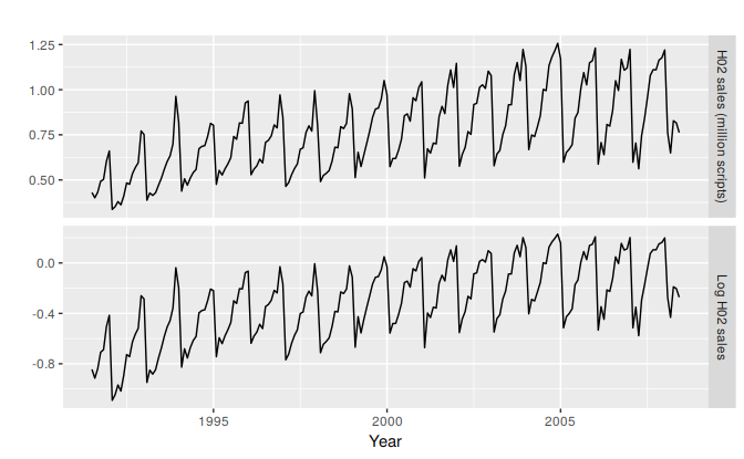

Figure 8.21: Cortecosteroid drug sales in Australia (in millions of scripts per month). Logged data shown in bottom panel.

Data from July 1991 to June 2008 are plotted in Figure 8.21. There is a small increase in the variance with the level, so we take logarithms to stabilize the variance.

The data are strongly seasonal and obviously non-stationary, so seasonal differencing will be used. The seasonally differenced data are shown in Figure 8.22. It is not clear at this point whether we should do another difference or not. We decide not to, but the choice is not obvious.

The last few observations appear to be different (more variable) from the earlier data. This may be due to the fact that data are sometimes revised when earlier sales are reported late.

lh02 %>% diff(lag=12) %>%
  ggtsdisplay(xlab="Year", main="Seasonally differenced H02 scripts")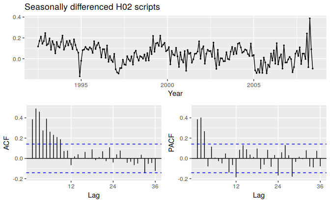

Figure 8.22: Seasonally differenced cortecosteroid drug sales in Australia (in millions of scripts per month).

In the plots of the seasonally differenced data, there are spikes in the PACF at lags 12 and 24, but nothing at seasonal lags in the ACF. This may be suggestive of a seasonal AR(2) term. In the non-seasonal lags, there are three significant spikes in the PACF, suggesting a possible AR(3) term. The pattern in the ACF is not indicative of any simple model.

Consequently, this initial analysis suggests that a possible model for these data is an ARIMA(3,0,0)(2,1,0)$_{12}$. We fit this model, along with some variations on it, and compute the AICc values shown in the following table.

Model	AICc
ARIMA(3,0,1)(0,1,2)$_{12}$	-485
ARIMA(3,0,1)(1,1,1)$_{12}$	-484
ARIMA(3,0,1)(0,1,1)$_{12}$	-484
ARIMA(3,0,1)(2,1,0)$_{12}$	-476
ARIMA(3,0,0)(2,1,0)$_{12}$	-475
ARIMA(3,0,2)(2,1,0)$_{12}$	-475
ARIMA(3,0,1)(1,1,0)$_{12}$	-463

Of these models, the best is the ARIMA(3,0,1)(0,1,2)$_{12}$ model (i.e., it has the smallest AICc value).

(fit <- Arima(h02, order=c(3,0,1), seasonal=c(0,1,2), lambda=0))
#> Series: h02 
#> ARIMA(3,0,1)(0,1,2)[12] 
#> Box Cox transformation: lambda= 0 
#> 
#> Coefficients:
#>          ar1    ar2    ar3    ma1    sma1    sma2
#>       -0.160  0.548  0.568  0.383  -0.522  -0.177
#> s.e.   0.164  0.088  0.094  0.190   0.086   0.087
#> 
#> sigma^2 estimated as 0.00428:  log likelihood=250
#> AIC=-486   AICc=-485   BIC=-463

checkresiduals(fit, lag=36)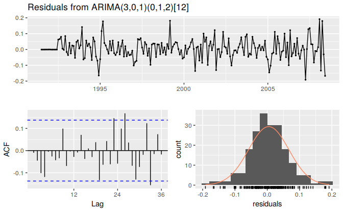

$Residuals from the ARIMA(3,0,1)(0,1,2)$_{12}$ model applied to the H02 monthly script sales data.$

Figure 8.23: Residuals from the ARIMA(3,0,1)(0,1,2)$_{12}$ model applied to the H02 monthly script sales data.

#> 
#>  Ljung-Box test
#> 
#> data:  Residuals from ARIMA(3,0,1)(0,1,2)[12]
#> Q* = 51, df = 30, p-value = 0.01
#> 
#> Model df: 6.   Total lags used: 36

The residuals from this model are shown in Figure 8.23. There are a few significant spikes in the ACF, and the model fails the Ljung-Box test. The model can still be used for forecasting, but the prediction intervals may not be accurate due to the correlated residuals.

Next we will try using the automatic ARIMA algorithm. Running auto.arima() with all arguments left at their default values led to an ARIMA(2,1,3)(0,1,1)$_{12}$ model. However, the model still fails the Ljung-Box test. Sometimes it is just not possible to find a model that passes all of the tests.

Test set evaluation:

We will compare some of the models fitted so far using a test set consisting of the last two years of data. Thus, we fit the models using data from July 1991 to June 2006, and forecast the script sales for July 2006 – June 2008. The results are summarised in the following table.

Model	RMSE
ARIMA(3,0,1)(0,1,2)$_{12}$	0.0622
ARIMA(3,0,1)(1,1,1)$_{12}$	0.0630
ARIMA(2,1,4)(0,1,1)$_{12}$	0.0632
ARIMA(2,1,3)(0,1,1)$_{12}$	0.0634
ARIMA(3,0,3)(0,1,1)$_{12}$	0.0639
ARIMA(2,1,5)(0,1,1)$_{12}$	0.0640
ARIMA(3,0,1)(0,1,1)$_{12}$	0.0644
ARIMA(3,0,2)(0,1,1)$_{12}$	0.0644
ARIMA(3,0,2)(2,1,0)$_{12}$	0.0645
ARIMA(3,0,1)(2,1,0)$_{12}$	0.0646
ARIMA(4,0,2)(0,1,1)$_{12}$	0.0648
ARIMA(4,0,3)(0,1,1)$_{12}$	0.0648
ARIMA(3,0,0)(2,1,0)$_{12}$	0.0661
ARIMA(3,0,1)(1,1,0)$_{12}$	0.0679

The models chosen manually and with auto.arima are both in the top four models based on their RMSE values.

When models are compared using AICc values, it is important that all models have the same orders of differencing. However, when comparing models using a test set, it does not matter how the forecasts were produced — the comparisons are always valid. Consequently, in the table above, we can include some models with only seasonal differencing and some models with both first and seasonal differencing, while in the earlier table containing AICc values, we only compared models with seasonal differencing but no first differencing.

None of the models considered here pass all of the residual tests. In practice, we would normally use the best model we could find, even if it did not pass all of the tests.

Forecasts from the ARIMA(3,0,1)(0,1,2)$_{12}$ model (which has the lowest RMSE value on the test set, and the best AICc value amongst models with only seasonal differencing) are shown in Figure 8.24.

h02 %>%
  Arima(order=c(3,0,1), seasonal=c(0,1,2), lambda=0) %>%
  forecast() %>%
  autoplot() +
    ylab("H02 sales (million scripts)") + xlab("Year")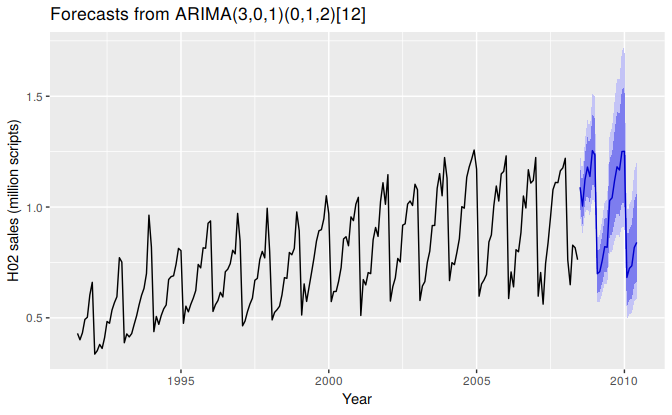

$Forecasts from the ARIMA(3,0,1)(0,1,2)$_{12}$ model applied to the H02 monthly script sales data.$

Figure 8.24: Forecasts from the ARIMA(3,0,1)(0,1,2)$_{12}$ model applied to the H02 monthly script sales data.

ARIMA	\(~\underbrace{(p, d, q)}\)	\(\underbrace{(P, D, Q)_{m}}\)
	\({\uparrow}\)	\({\uparrow}\)
	Non-seasonal part	Seasonal part of
	of the model	of the model

Model	AICc
ARIMA(3,0,1)(0,1,2)\(_{12}\)	-485
ARIMA(3,0,1)(1,1,1)\(_{12}\)	-484
ARIMA(3,0,1)(0,1,1)\(_{12}\)	-484
ARIMA(3,0,1)(2,1,0)\(_{12}\)	-476
ARIMA(3,0,0)(2,1,0)\(_{12}\)	-475
ARIMA(3,0,2)(2,1,0)\(_{12}\)	-475
ARIMA(3,0,1)(1,1,0)\(_{12}\)	-463