1.7 The statistical forecasting perspective

The thing we are trying to forecast is unknown (or we wouldn’t be forecasting it), and so we can think of it as a random variable. For example, the total sales for next month could take a range of possible values, and until we add up the actual sales at the end of the month, we don’t know what the value will be. So until we know the sales for next month, it is a random quantity.

Because next month is relatively close, we usually have a good idea what the likely sales values could be. On the other hand, if we are forecasting the sales for the same month next year, the possible values it could take are much more variable. In most forecasting situations, the variation associated with the thing we are forecasting will shrink as the event approaches. In other words, the further ahead we forecast, the more uncertain we are.

We can imagine many possible futures, each yielding a different value for the thing we wish to forecast. Plotted below in black are the total international visitors to Australia from 1980 to 2015. Also shown are ten possible futures from 2016–2025.

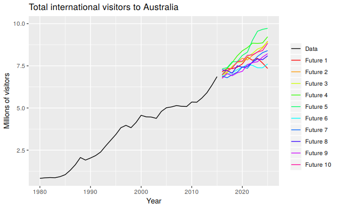
Figure 1.2: Total international visitors to Australia (1980-2015) along with ten possible futures.

When we obtain a forecast, we are estimating the middle of the range of possible values the random variable could take. Very often, a forecast is accompanied by a prediction interval giving a range of values the random variable could take with relatively high probability. For example, a 95% prediction interval contains a range of values which should include the actual future value with probability 95%.

Instead of plotting individual possible futures as shown in Figure 1.2, we normally show these prediction intervals instead. The plot below shows 80% and 95% intervals for the future Australian international visitors. The blue line is the average of the possible future values, which we call the “point forecasts”.

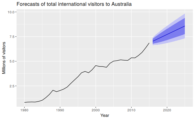
Figure 1.3: Total international visitors to Australia (1980–2015) along with 10-year forecasts and 80% and 95% prediction intervals.

We will use the subscript \(t\) for time. For example, \(y_t\) will denote the observation at time \(t\). Suppose we denote all the information we have observed as \({\cal I}\) and we want to forecast \(y_t\). We then write \(y_{t} | {\cal I}\) meaning “the random variable \(y_{t}\) given what we know in \({\cal I}\)”. The set of values that this random variable could take, along with their relative probabilities, is known as the “probability distribution” of \(y_{t} |{\cal I}\). In forecasting, we call this the “forecast distribution”.

When we talk about the “forecast”, we usually mean the average value of the forecast distribution, and we put a “hat” over \(y\) to show this. Thus, we write the forecast of \(y_t\) as \(\hat{y}_t\), meaning the average of the possible values that \(y_t\) could take given everything we know. Occasionally, we will use \(\hat{y}_t\) to refer to the median (or middle value) of the forecast distribution instead.

It is often useful to specify exactly what information we have used in calculating the forecast. Then we will write, for example, \(\hat{y}_{t|t-1}\) to mean the forecast of \(y_t\) taking account of all previous observations \((y_1,\dots,y_{t-1})\). Similarly, \(\hat{y}_{T+h|T}\) means the forecast of \(y_{T+h}\) taking account of \(y_1,\dots,y_T\) (i.e., an \(h\)-step forecast taking account of all observations up to time \(T\)).