7.4 A taxonomy of exponential smoothing methods

Exponential smoothing methods are not restricted to those we have presented so far. By considering variations in the combinations of the trend and seasonal components, nine exponential smoothing methods are possible, listed in Table 7.6. Each method is labelled by a pair of letters (T,S) defining the type of ‘Trend’ and ‘Seasonal’ components. For example, (A,M) is the method with an additive trend and multiplicative seasonality; (A_d,N) is the method with damped trend and no seasonality; and so on.

Table 7.6: A two-way classification of exponential smoothing methods.
Trend Component	Seasonal	Component
	N (None)	A (Additive)	M (Multiplicative)
N (None)	(N,N)	(N,A)	(N,M)
A (Additive)	(A,N)	(A,A)	(A,M)
A_d (Additive damped)	(A_d,N)	(A_d,A)	(A_d)

Some of these methods we have already seen:

Short hand	Method
(N,N)	Simple exponential smoothing
(A,N)	Holt’s linear method
(A_d,N)	Additive damped trend method
(A,A)	Additive Holt-Winters’ method
(A,M)	Multiplicative Holt-Winters’ method
(A_d,M)	Holt-Winters’ damped method

This type of classification was first proposed by Pegels (1969), who also included a method with a multiplicative trend. It was later extended by Gardner Jr (1985) to include methods with an additive damped trend and by Taylor (2003) to include methods with a multiplicative damped trend. We do not consider the multiplicative trend methods in this book as they tend to produce poor forecasts. See Rob J Hyndman et al. (2008) for a more thorough discussion of all exponential smoothing methods.

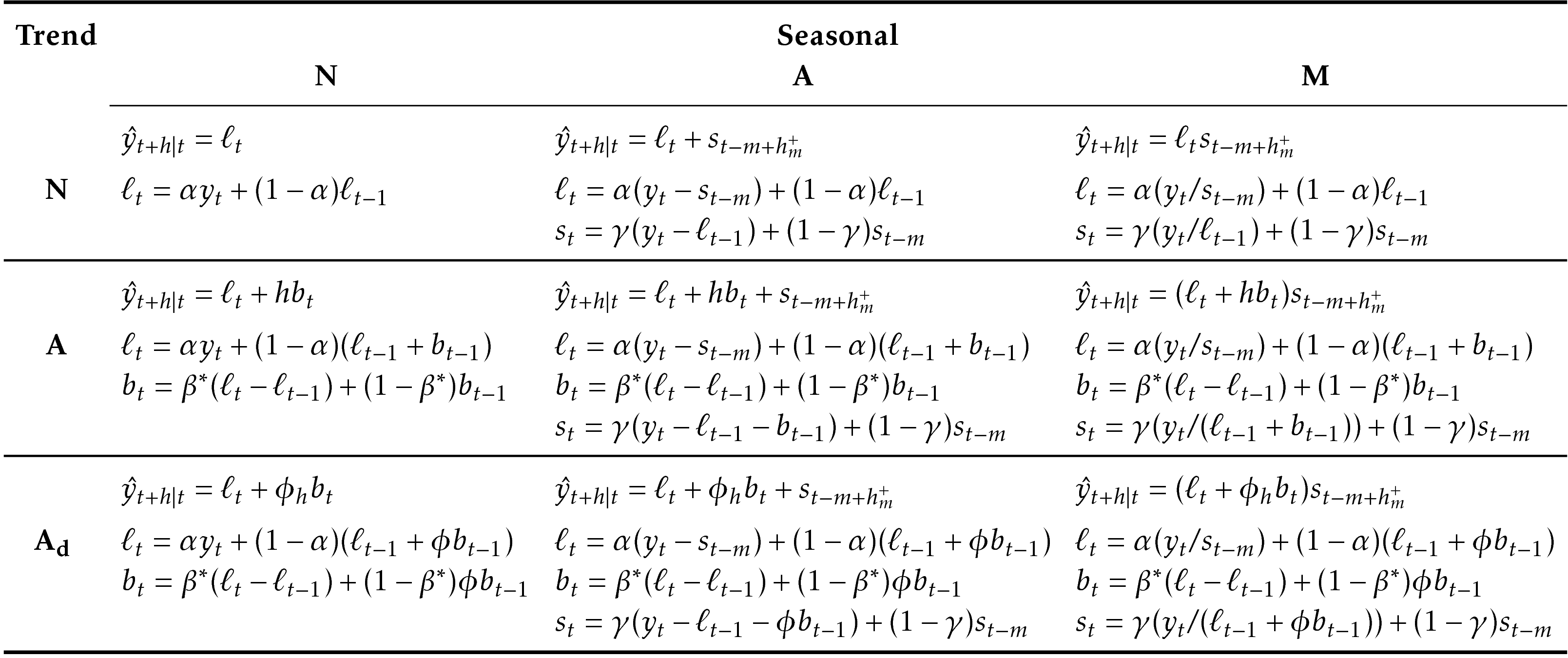
Table 7.7 gives the recursive formulae for applying the nine exponential smoothing methods in Table 7.6. Each cell includes the forecast equation for generating \(h\)-step-ahead forecasts, and the smoothing equations for applying the method.

Table 7.7: Formulae for recursive calculations and point forecasts. In each case, \(\ell_t\) denotes the series level at time \(t\), \(b_t\) denotes the slope at time \(t\), \(s_t\) denotes the seasonal component of the series at time \(t\), and \(m\) denotes the number of seasons in a year; \(\alpha\), \(\beta^*\), \(\gamma\) and \(\phi\) are smoothing parameters, \(\phi_h = \phi+\phi^2+\dots+\phi^{h}\) and \(h_m^+ = \lfloor(h-1) / m\rfloor + 1\).

References

Gardner Jr, Everette S. 1985. “Exponential Smoothing: The State of the Art” 4 (1): 1–28.

Hyndman, Rob J, Anne B Koehler, J Keith Ord, and Ralph D Snyder. 2008. Forecasting with Exponential Smoothing: The State Space Approach. Berlin: Springer-Verlag. www.exponentialsmoothing.net.

Pegels, C C. 1969. “Exponential Smoothing: Some New Variations.” Management Science 12: 311–15.

Taylor, J W. 2003. “Exponential Smoothing with a Damped Multiplicative Trend.” International Journal of Forecasting 19: 715–25.