6.8 Exercises
Show that a \(3\times5\) MA is equivalent to a 7-term weighted moving average with weights of 0.067, 0.133, 0.200, 0.200, 0.200, 0.133, and 0.067.
- The
plasticsdata set consists of the monthly sales (in thousands) of product A for a plastics manufacturer for five years.- Plot the time series of sales of product A. Can you identify seasonal fluctuations and/or a trend-cycle?
- Use a classical multiplicative decomposition to calculate the trend-cycle and seasonal indices.
- Do the results support the graphical interpretation from part (a)?
- Compute and plot the seasonally adjusted data.
- Change one observation to be an outlier (e.g., add 500 to one observation), and recompute the seasonally adjusted data. What is the effect of the outlier?
- Does it make any difference if the outlier is near the end rather than in the middle of the time series?
Recall your retail time series data (from Exercise 3 in Section 2.10). Decompose the series using X11. Does it reveal any outliers, or unusual features that you had not noticed previously?
Figures 6.16 and 6.17 shows the result of decomposing the number of persons in the civilian labor force in Australia each month from February 1978 to August 1995.
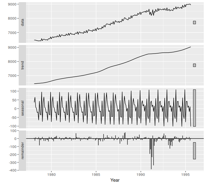
Figure 6.16: Decomposition of the number of persons in the civilian labor force in Australia each month from February 1978 to August 1995.
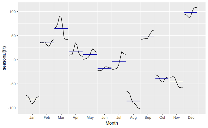
Figure 6.17: Seasonal component from the decomposition shown in Figure 6.16.
- Write about 3–5 sentences describing the results of the seasonal adjustment. Pay particular attention to the scales of the graphs in making your interpretation.
- Is the recession of 1991/1992 visible in the estimated components?
- This exercise uses the
cangasdata (monthly Canadian gas production in billions of cubic metres, January 1960 – February 2005).- Plot the data using
autoplot,ggsubseriesplotandggseasonplotto look at the effect of the changing seasonality over time. What do you think is causing it to change so much? - Do an STL decomposition of the data. You will need to choose
s.windowto allow for the changing shape of the seasonal component. - Compare the results with those obtained using SEATS and X11. How are they different?
- Plot the data using
- We will use the
bricksqdata (Australian quarterly clay brick production. 1956–1994) for this exercise.- Use an STL decomposition to calculate the trend-cycle and seasonal indices. (Experiment with having fixed or changing seasonality.)
- Compute and plot the seasonally adjusted data.
- Use a naïve method to produce forecasts of the seasonally adjusted data.
- Use
stlfto reseasonalize the results, giving forecasts for the original data. - Do the residuals look uncorrelated?
- Repeat with a robust STL decomposition. Does it make much difference?
- Compare forecasts from
stlfwith those fromsnaive, using a test set comprising the last 2 years of data. Which is better?
Use
stlfto produce forecasts of thewritingseries with eithermethod="naive"ormethod="rwdrift", whichever is most appropriate. Use thelambdaargument if you think a Box-Cox transformation is required.Use
stlfto produce forecasts of thefancyseries with eithermethod="naive"ormethod="rwdrift", whichever is most appropriate. Use thelambdaargument if you think a Box-Cox transformation is required.