11.1 Complex seasonality
So far, we have considered relatively simple seasonal patterns such as quarterly and monthly data. However, higher frequency data often exhibits more complicated seasonal patterns. For example, daily data may have a weekly pattern as well as an annual pattern. Hourly data usually has three types of seasonality: a daily pattern, a weekly pattern, and an annual pattern. Even weekly data can be difficult as it typically has an annual pattern with seasonal period of \(365.25/7\approx 52.179\) on average.
Such multiple seasonal patterns are becoming more common with high frequency data recording. Further examples where multiple seasonal patterns can occur include call volume in call centres, daily hospital admissions, requests for cash at ATMs, electricity and water usage, and access to computer web sites.
Most of the methods we have considered so far are unable to deal with these seasonal complexities. Even the ts class in R can only handle one type of seasonality, which is usually assumed to take integer values.
To deal with such series, we will use the msts class which handles multiple seasonality time series. Then you can specify all of the frequencies that might be relevant. It is also flexible enough to handle non-integer frequencies.
You won’t necessarily want to include all of these frequencies — just the ones that are likely to be present in the data. For example, if you have only 180 days of data, you can probably ignore the annual seasonality. If the data are measurements of a natural phenomenon (e.g., temperature), you might also be able to ignore the weekly seasonality.
Figure 11.1 shows the number of retail banking call arrivals per 5-minute interval between 7:00am and 9:05pm each weekday over a 33 week period. There is a strong daily seasonal pattern with frequency 169, and a weak weekly seasonal pattern with frequency \(169 \times 5=845\). (Call volumes on Mondays tend to be higher than the rest of the week.) If a longer series of data were available, there may also be an annual seasonal pattern.
p1 <- autoplot(calls) +
  ylab("Call volume") + xlab("Weeks") +
  scale_x_continuous(breaks=seq(1,33,by=2))
p2 <- autoplot(window(calls, end=4)) +
  ylab("Call volume") + xlab("Weeks") +
  scale_x_continuous(minor_breaks = seq(1,4,by=0.2))
gridExtra::grid.arrange(p1,p2)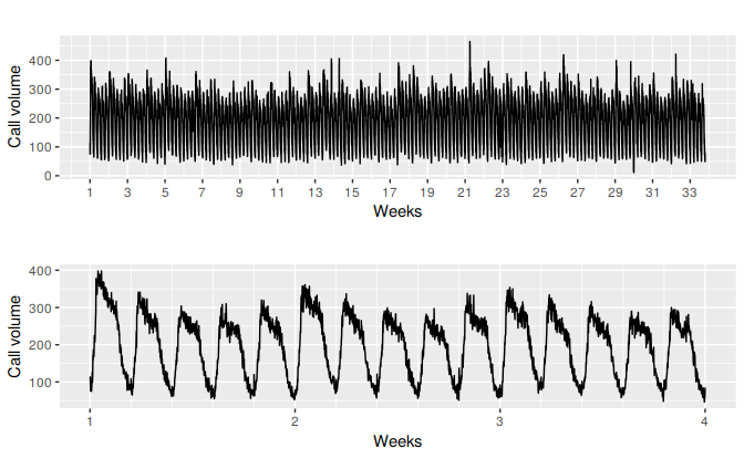
Figure 11.1: Five-minute call volume handled on weekdays between 7am and 9:05pm in a large North American commercial bank. Top panel shows data from 3 March 2003 to 23 May 2003. Bottom panel shows only the first three weeks.
Dynamic harmonic regression with multiple seasonal periods
With multiple seasonalities, we can use Fourier terms as we did in earlier chapters. Because there are multiple seasonalities, we need to add Fourier terms for each seasonal period. In this case, the seasonal periods are 169 and 845, so the Fourier terms are of the form
\[
\sin\left(\frac{2\pi kt}{169}\right), \qquad
\cos\left(\frac{2\pi kt}{169}\right), \qquad
\sin\left(\frac{2\pi kt}{845}\right), \qquad \text{and}
\cos\left(\frac{2\pi kt}{845}\right),
\]
for \(k=1,2,\dots\). The fourier function can generate these for you.
We will fit a dynamic regression model with an ARMA error structure. The total number of Fourier terms for each seasonal period have been chosen to minimize the AICc. We will use a log transformation (lambda=0) to ensure the forecasts and prediction intervals remain positive.
#fit <- auto.arima(calls, seasonal=FALSE, lambda=0,
#         xreg=fourier(calls, K=c(10,10)))
#fc <- forecast(fit, xreg=fourier(calls, K=c(10,10), h=2*169))
#autoplot(fc, include=5*169) +
#  ylab("Call volume") + xlab("Weeks")
This is a very large model (containing 120+??=?? parameters).
TBATS models
An alternative approach developed by De Livera, Hyndman, and Snyder (2011) uses a combination of Fourier terms with an exponential smoothing state space model and a Box-Cox transformation, in a completed automated manner. As with any automated modelling framework, it does not always work, but it can be a useful approach in some circumstances.
A TBATS model differs from dynamic harmonic regression in that the seasonality is allowed to change slowly over time in a TBATS model, while harmonic regression terms force the seasonal patterns to repeat periodically without changing. One drawback of TBATS models is that they can be very slow to estimate, especially with long time series. So we will consider a subset of the calls data to save time.
calls %>%
  subset(start=length(calls)-1000) %>%
  tbats -> fit2
fc2 <- forecast(fit2, h=2*169)
autoplot(fc2, include=5*169) +
  ylab("Call volume") + xlab("Weeks")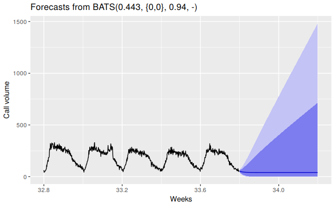
Complex seasonality with covariates
TBATS models do not allow for covariates, although they can be included in dynamic harmonic regression models. One common application of such models is electricity demand modelling.
Figure 11.2 shows half-hourly electricity demand in Victoria, Australia, during 2014, along with temperatures in the same period.
autoplot(elecdemand[,c("Demand","Temperature")], facet=TRUE) +
  scale_x_continuous(minor_breaks=NULL,
    breaks=2014+cumsum(c(0,31,28,31,30,31,30,31,31,30,31,30))/365,
    labels=month.abb) +
  xlab("Time") + ylab("")
#> Warning: Ignoring unknown parameters: series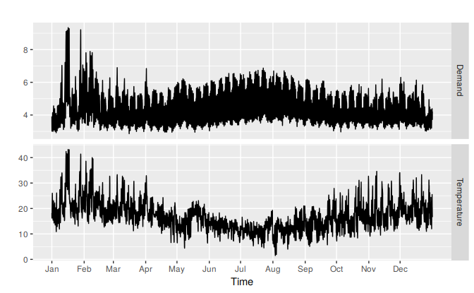
Figure 11.2: Half-hourly electricity demand and corresponding temperatures in 2014, Victoria, Australia.
Plotting electricity demand against temperature shows that there is a nonlinear relationship between the two, with demand increasing for low temperatures (due to heating) and increasing for high temperatures (due to cooling).
elecdemand %>%
  as.data.frame %>%
  ggplot(aes(x=Temperature, y=Demand)) + geom_point() +
    xlab("Temperature (degrees Celsius)") +
    ylab("Demand (GW)")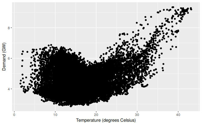
We will fit a regression model with a piecewise linear function of temperature (containing a knot at 18 degrees), and harmonic regression terms to allow for the daily seasonal pattern.
cooling <- pmax(elecdemand[,"Temperature"], 18)
fit <- auto.arima(elecdemand[,"Demand"],
         xreg = cbind(fourier(elecdemand, c(10,10,0)),
               heating=elecdemand[,"Temperature"],
               cooling=cooling))
Forecasting with such models is difficult because we require future values of the predictor variables. Future values of the Fourier terms are easy to compute, but future temperatures are, of course, unknown. We could use temperature forecasts obtain from a meteorological model if we are only interested in forecasting up to a week ahead. Alternatively, we could use scenario forecasting and plug in possible temperature patterns. In the following example, we have used a repeat of the last week of temperatures to generate future possible demand values.
#temps <- subset(elecdemand[,"Temperature"], start=NROW(elecdemand)-7*48-1)
#fc <- forecast(fit, xreg=cbind(fourier(temps, c(10,10,0)),
#                           heating=temps, cooling=pmax(temps,18)))
#autoplot(fc)#checkresiduals(fc)References
De Livera, Alysha M, Rob J Hyndman, and Ralph D Snyder. 2011. “Forecasting Time Series with Complex Seasonal Patterns Using Exponential Smoothing.” Journal of the American Statistical Association 106 (496): 1513–27.