10.1 Hierarchical time series
Time series can often be naturally disaggregated by various attributes of interest. For example, the total number of bicycles sold by a cycling manufacturer can be disaggregated by product type such as: road bikes, mountain bikes, children bikes and hybrids. Each of these can be disaggregated into finer categories. For example children’s bikes can be divided into balance bikes for children under the age of four, single speed bikes for children between the ages of four and six and other bikes for children over the age of six. Hybrid bikes can be divided into city, commuting, comfort, and trekking bikes; and so on. Such a collection of time series follow a hierarchical aggregation structure and we refer to these as hierarchical time series.
Commonly found in business and economics are hierarchical time series based on geographical locations. For example the total sales of a manufacturing company can be disaggregated by country, then within each country by state, within each state by region and so on down to the outlet level.
A feature that distinguishes hierarchical time series (from grouped time series that follow in Section 10.2) is that they have a unique structure with which they aggregate. Figure 10.1 shows a \(K=2\)-level hierarchical structure. At the top of the hierarchy, at level 0, is the “Total”, the most aggregate level of the data. We denote as \(y_t\) the \(t\)th observation of the “Total” series for \(t=1,\dots,T\). The “Total” is disaggregated into two series at level 1 and each of these into three and two series respectively at the bottom-level of the hierarchy. Below the top most aggregate level, we denote as \(\y{j}{t}\) the \(t\)th observation of the series which corresponds to node \(j\). For example \(y_{A,t}\) denotes the \(t\)th observation of the series corresponding to node A at level 1, \(y_{AB,t}\) denotes the \(t\)th observation of the series corresponding to node AB at level 2, and so on.
The total number of series in the hierarchy is \(n=1+2+5=8\). We denote as \(m\) the number of series at the bottom-level, a dimension that is important in what follows. In this case \(m=5\). Note that always \(n>m\).
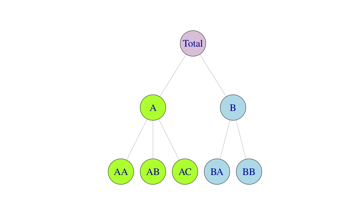
Figure 10.1: A two level hierarchical tree diagram.
For any time \(t\), the observations at the bottom-level of the hierarchy will aggregate to the observations of the series above. For example, \[\begin{equation} y_{t}=\y{AA}{t}+\y{AB}{t}+\y{AC}{t}+\y{BA}{t}+\y{BB}{t} \tag{10.1} \end{equation}\] and \[\begin{equation} \y{A}{t}=\y{AA}{t}+\y{AB}{t}+\y{AC}{t}\quad \text{and} \quad \y{B}{t}=\y{BA}{t}+\y{BB}{t}. \tag{10.2} \end{equation}\] Substituting (10.2) into (10.1) we also get \(y_{t}=\y{A}{t}+\y{B}{t}\). These equations can be thought of as aggregation constraints or summing equalities and can be more efficienlty represented using matrix notation. We construct an \(n\times m\) matrix \(\bm{S}\) referred to as the summing matrix which dictates how the bottom-level series are aggregated, consistent with the aggregation structure. For the hierarchical structure in Figure 10.1 we write \[ \begin{bmatrix} y_{t} \\ \y{A}{t} \\ \y{B}{t} \\ \y{AA}{t} \\ \y{AB}{t} \\ \y{AC}{t} \\ \y{BA}{t} \\ \y{BB}{t} \end{bmatrix} = \begin{bmatrix} 1 & 1 & 1 & 1 & 1 \\ 1 & 1 & 1 & 0 & 0 \\ 0 & 0 & 0 & 1 & 1 \\ 1 & 0 & 0 & 0 & 0 \\ 0 & 1 & 0 & 0 & 0 \\ 0 & 0 & 1 & 0 & 0 \\ 0 & 0 & 0 & 1 & 0 \\ 0 & 0 & 0 & 0 & 1 \end{bmatrix} \begin{bmatrix} \y{AA}{t} \\ \y{AB}{t} \\ \y{AC}{t} \\ \y{BA}{t} \\ \y{BB}{t} \end{bmatrix} \] or in more compact notation \[\begin{equation} \bm{y}_t=\bm{S}\bm{y}_{K,t}, \tag{10.3} \end{equation}\] where \(\bm{y}_t\) is a \(n\)-dimensional vector of all the observations in the hierarchy at time \(t\), \(\bm{S}\) is the summing matrix as defined above, and \(\bm{y}_{K,t}\) is an \(m\)-dimensional vector of all the observations in the bottom-level of the hierarchy at time \(t\). Note that the first row in the summing \(\bm{S}\) represents equation (10.1) above, the second and third row represent (10.2). The rows below these comprise an \(m\)-dimensional identity matrix \(\bm{I}_m\) so that each bottom-level observation on the right hand side of the equation is equal to itself in the left hand side.
Example: Australian tourism hierarchy
Australia is divided into eight geographical areas (some referred to as states and others as territories) with each one having its own government and some economic and administrative autonomy. Each of these can be further subdivided into smaller areas of interest referred to as zones. Business planners and tourism authorities are interested in forecasts for the whole of Australia, the states and the territories, and also the regions. In this example we concentrate on quarterly domestic tourism demand, measured as the number of visitor nights Australians spend away from home, for the six states of Australia, namely: New South Wales (NSW), Queensland (QLD), South Australia (SAU), Victoria (VIC), Western Australia (WA) and other (OTH). For each of these we consider visitor nights within the following zones.
| State | Zones |
|---|---|
| NSW | Metro (NSWMetro), North Coast (NSWNthCo), South Coast (NSWSthCo), South Inner (NSWSthIn), North Inner (NSWNthIn) |
| QLD | Metro (QLDMetro), Central (QLDCntrl), North Coast (QLDNthCo) |
| SAu | Metro (SAUMetro), Costal (SAUCoast), Inner (SAUInner) |
| VIC | Metro (VICMetro), West Coast (VICWstCo), East Coast (VICEstCo), Inner (VICInner) |
| WAu | Metro (WAUMetro), Costal (WAUCoast), Inner (WAUInner) |
| OTH | Metro (OTHMetro), Non-Metro (OTHNoMet) |
In summary, we consider five zones for NSW, four zones for VIC, and three zones for each QLD, SAU and WAU. Note that Metro zones contain the capital cities and surrounding areas around these generally considered to be metro areas. For OTH we consider Metro (OTHMetro) and non-Metro (OTHNoMet) areas across the rest of Australia. For further details on these geographical areas please refer to Appendix C in Wickramasuriya, Athanasopoulos, and Hyndman (2015).
To create a hierarchical time series we use the hts function as shown in the code below. The function requires as inputs the bottom-level time series and information about the hierarchical structure. vn2 is a time series matrix containing the bottom-level series. There are alternative ways to pass to the function the structure of the hieararchy. In this case we are using the characters input. The first three characters of each column name of vn2 capture the categories at the first level of the hierarchy (States). The following five characters capture the bottom-level categories (Zones).
vn2 <- read.csv("Ch10Data/vn2.csv")
vn2 <- ts(vn2, start = 1998, frequency = 4)
require(hts)
tourism.hts <- hts(vn2, characters = c(3, 5))
# I keep vn2 here as we will only use this line when we add vn2 in the fpp2 package
The top plot in Figure 10.2 shows the total number of visitor nights for the total of Australia while the plots bellow show the visitor nights disaggregated by state. These reveal diverse and rich dynamics at the aggregate national level and the first level of disaggregation across each state. The aggts function extracts time series from a hts object for any level of aggregation.
tourismL0 <- aggts(tourism.hts, levels = 0)
p1<-autoplot(tourismL0) +
  xlab("Year") +
  ylab("Visitor nights ('000)")+
  ggtitle("Total")

tourismL1 <- aggts(tourism.hts, levels = 1)
p2<-autoplot(tourismL1[,c(1,3,5)]) +
  xlab("Year") +
  ylab("Visitor nights ('000)")+
  scale_colour_discrete(guide = guide_legend(title = "State"))

p3<-autoplot(tourismL1[,c(2,4,6)]) +
  xlab("Year") +
  ylab("Visitor nights ('000)")+
  scale_colour_discrete(guide = guide_legend(title = "State"))

lay=rbind(c(1,1),c(2,3))
gridExtra::grid.arrange(p1, p2,p3, layout_matrix=lay)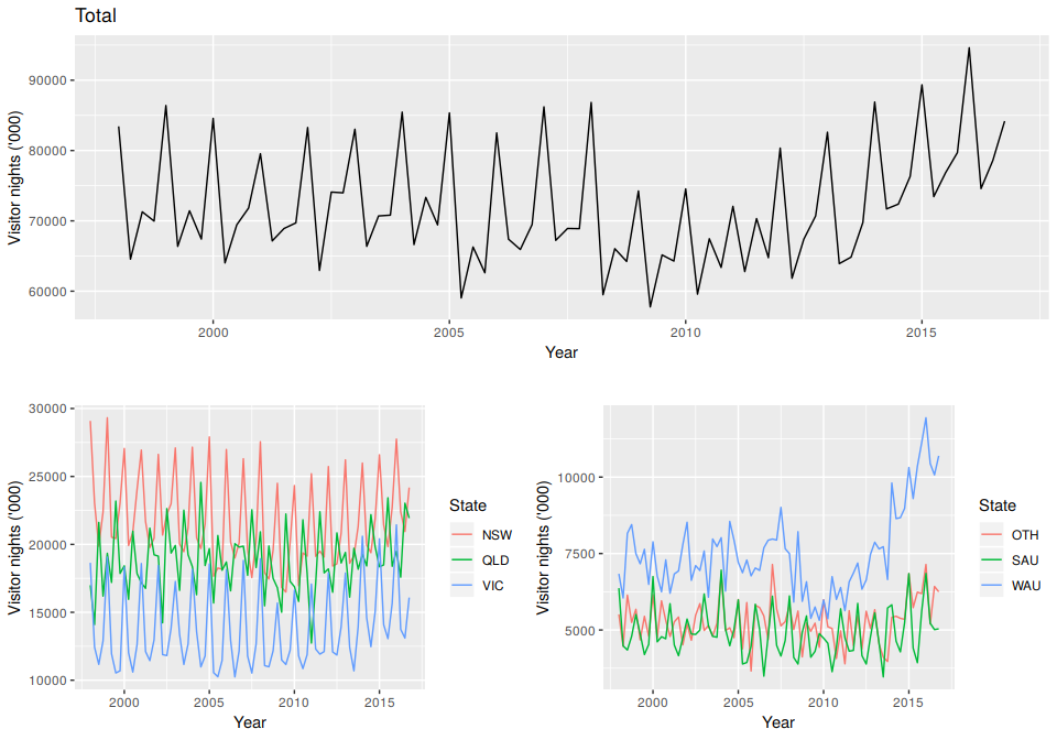
Figure 10.2: Australian domestic visitor nights over the period 1998 Q1 to 2016 Q4 disaggregated by State.
The plots in Figure 10.3 below show the bottom-level time series, i.e., the visitor nights for each zone. These help us visualise the diverse individual dynamics within each zones and assist in identifying unique and important time series. Notice for example the costal WAU zone which shows significant growth over the last few years.
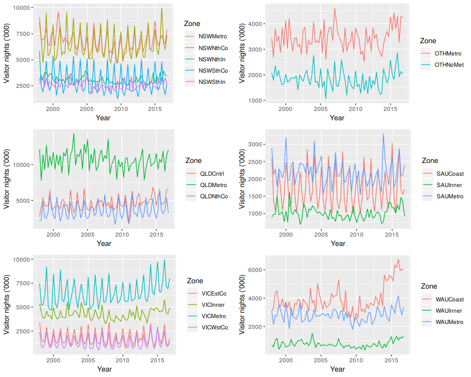
Figure 10.3: Australian domestic visitor nights over the period 1998 Q1 to 2016 Q4 disaggregated by Zones.
References
Wickramasuriya, Shanika L, George Athanasopoulos, and Rob J Hyndman. 2015. “Forecasting Hierarchical and Grouped Time Series Through Trace Minimization.” Working paper 15/15. Monash University Econometrics & Business Statistics.