6.3 Classical decomposition
The classical decomposition method originated in the 1920s. It is a relatively simple procedure, and forms the starting point for most other methods of time series decomposition. There are two forms of classical decomposition: an additive decomposition and a multiplicative decomposition. These are described below for a time series with seasonal period \(m\) (e.g., \(m=4\) for quarterly data, \(m=12\) for monthly data, \(m=7\) for daily data with a weekly pattern).
In classical decomposition, we assume that the seasonal component is constant from year to year. For multiplicative seasonality, the \(m\) values that form the seasonal component are sometimes called the “seasonal indices”.
Additive decomposition
- Step 1
- If \(m\) is an even number, compute the trend-cycle component using a \(2\times m\)-MA to obtain \(\hat{T}_t\). If \(m\) is an odd number, compute the trend-cycle component using an \(m\)-MA to obtain \(\hat{T}_t\).
- Step 2
- Calculate the detrended series: \(y_t - \hat{T}_t\).
- Step 3
- To estimate the seasonal component for each season, simply average the detrended values for that season. For example, with monthly data, the seasonal component for March is the average of all the detrended March values in the data. These seasonal component values are then adjusted to ensure that they add to zero. The seasonal component is obtained by stringing together these values for each year of data. This gives \(\hat{S}_t\).
- Step 4
- The remainder component is calculated by subtracting the estimated seasonal and trend-cycle components: \(\hat{R}_t = y_t - \hat{T}_t - \hat{S}_t\).
Multiplicative decomposition
A classical multiplicative decomposition is very similar, except that the subtractions are replaced by divisions.
- Step 1
- If \(m\) is an even number, compute the trend-cycle component using a \(2\times m\)-MA to obtain \(\hat{T}_t\). If \(m\) is an odd number, compute the trend-cycle component using an \(m\)-MA to obtain \(\hat{T}_t\).
- Step 2
- Calculate the detrended series: \(y_t/ \hat{T}_t\).
- Step 3
- To estimate the seasonal component for each season, simply average the detrended values for that season. For example, with monthly data, the seasonal index for March is the average of all the detrended March values in the data. These seasonal indexes are then adjusted to ensure that they add to \(m\). The seasonal component is obtained by stringing together all of the seasonal indices for each year of data. This gives \(\hat{S}_t\).
- Step 4
- The remainder component is calculated by dividing out the estimated seasonal and trend-cycle components: \(\hat{R}_{t} = y_t /( \hat{T}_t \hat{S}_t)\).
elecequip %>% decompose(type="multiplicative") %>%
  autoplot() + xlab("Year") +
  ggtitle("Classical multiplicative decomposition of electrical equipment index")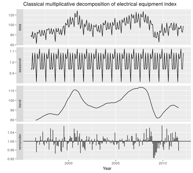
Figure 6.8: A classical multiplicative decomposition of the new orders index for electrical equipment.
Figure 6.8 shows a classical decomposition of the electrical equipment index. Compare this decomposition with that shown in Figure 6.1. The run of large negative remainder values in 2009 suggests that there is some “leakage” of the trend-cycle component into the remainder component. The trend-cycle estimate has over-smoothed the drop in the data, and the corresponding remainder values have been affected by the poor trend-cycle estimate.
Comments on classical decomposition
While classical decomposition is still widely used, it is not recommended, as there are now several much better methods. Some of the problems with classical decomposition are summarised below.
The estimate of the trend-cycle is unavailable for the first few and last few observations. For example, if \(m=12\), there is no trend-cycle estimate for the first six or the last six observations. Consequently, there is also no estimate of the remainder component for the same time periods.
The trend-cycle estimate tends to over-smooth rapid rises and falls in the data (as seen in the above example).
Classical decomposition methods assume that the seasonal component repeats from year to year. For many series, this is a reasonable assumption, but for some longer series it is not. For example, electricity demand patterns have changed over time as air conditioning has become more widespread. Specifically, in many locations, the seasonal usage pattern from several decades ago had its maximum demand in winter (due to heating), while the current seasonal pattern has its maximum demand in summer (due to air conditioning). The classical decomposition methods are unable to capture these seasonal changes over time.
Occasionally, the values of the time series in a small number of periods may be particularly unusual. For example, the monthly air passenger traffic may be affected by an industrial dispute, making the traffic during the dispute very different from usual. The classical method is not robust to these kinds of unusual values.