7.5 Innovations state space models for exponential smoothing
In the rest of this chapter, we study the statistical models that underlie the exponential smoothing methods we have considered so far. The exponential smoothing methods presented in Table 7.7 are algorithms which generate point forecasts. The statistical models in this section generate the same point forecasts, but can also generate prediction (or forecast) intervals. A statistical model is a stochastic (or random) data generating process that can produce an entire forecast distribution. The general statistical framework we will introduce also provides a way of using the model selection criteria introduced in Chapter 5, thus allowing the choice of model to be made in an objective manner.
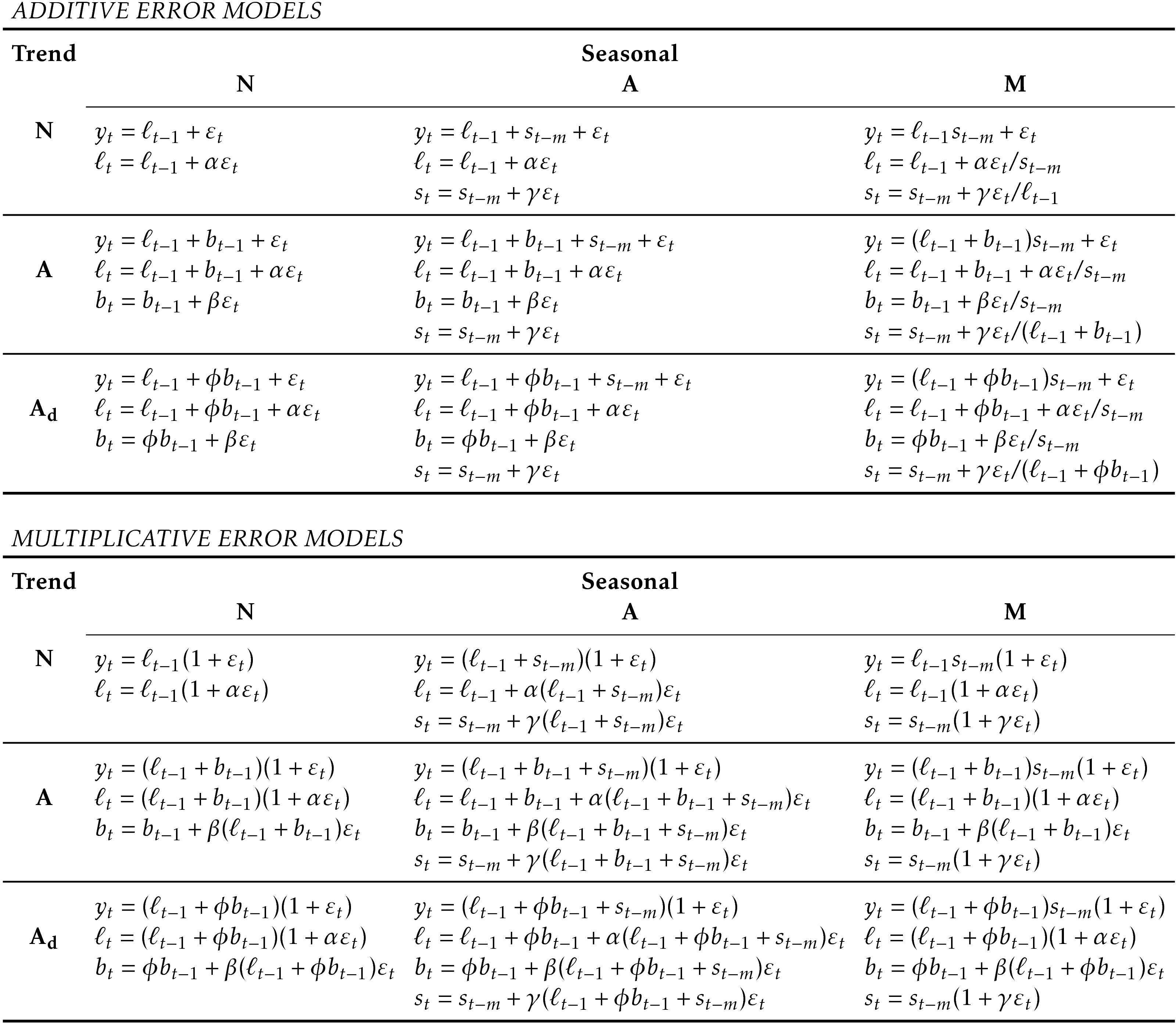
Each model consists of a measurement equation that describes the observed data, and some transition equations that describe how the unobserved components or states (level, trend, seasonal) change over time. Hence, these are referred to as “state space models”.
For each method there exist two models: one with additive errors and one with multiplicative errors. The point forecasts produced by the models are identical if they use the same smoothing parameter values. They will, however, generate different prediction intervals.
To distinguish between a model with additive errors and one with multiplicative errors (and also to distinguish the models from the methods), we add a third letter to the classification of Table 7.6. We label each state space model as ETS(\(\cdot,\cdot,\cdot\)) for (Error, Trend, Seasonal). This label can also be thought of as ExponenTial Smoothing. Using the same notation as in Table 7.6, the possibilities for each component are: Error \(=\{\)A,M\(\}\), Trend \(=\{\)N,A,Ad\(\}\) and Seasonal \(=\{\)N,A,M\(\}\).
ETS(A,N,N): simple exponential smoothing with additive errors
Recall the component form of simple exponential smoothing: \[\begin{align*} \text{Forecast equation} && \hat{y}_{t+1|t} & = \ell_{t}\\ \text{Smoothing equation} && \ell_{t} & = \alpha y_{t} + (1 - \alpha)\ell_{t-1}, \end{align*}\] If we re-arrange the smoothing equation for the level, we get the error correction form: \[\begin{align*} \ell_{t} %&= \alpha y_{t}+\ell_{t-1}-\alpha\ell_{t-1}\\ &= \ell_{t-1}+\alpha( y_{t}-\ell_{t-1})\\ &= \ell_{t-1}+\alpha e_{t} \end{align*}\] where \(e_{t}=y_{t}-\ell_{t-1}=y_{t}-\hat{y}_{t|t-1}\) for \(t=1,\dots,T\). That is, \(e_{t}\) is the one-step error at time \(t\) computed on the training data.
The training data errors lead to the adjustment of the estimated level throughout the smoothing process for \(t=1,\dots,T\). For example, if the error at time \(t\) is negative, then \(\hat{y}_{t|t-1}>y_t\) and so the level at time \(t-1\) has been over-estimated. The new level \(\ell_t\) is then the previous level \(\ell_{t-1}\) adjusted downwards. The closer \(\alpha\) is to one, the “rougher” the estimate of the level (large adjustments take place). The smaller the \(\alpha\), the “smoother” the level (small adjustments take place).
We can also write \(y_t = \ell_{t-1} + e_t\), so that each observation is equal to the previous level plus an error. To make this into an innovations state space model, all we need to do is specify the probability distribution for \(e_t\). For a model with additive errors, we assume that one-step forecast errors \(e_t\) are normally distributed white noise with mean 0 and variance \(\sigma^2\). A short-hand notation for this is \(e_t = \varepsilon_t\sim\text{NID}(0,\sigma^2)\); NID stands for “normally and independently distributed”.
Then the equations of the model can be written as \[\begin{align} y_t &= \ell_{t-1} + \varepsilon_t \tag{7.3}\\ \ell_t&=\ell_{t-1}+\alpha \varepsilon_t. \tag{7.4} \end{align}\] We refer to (7.3) as the measurement (or observation) equation and (7.4) as the state (or transition) equation. These two equations, together with the statistical distribution of the errors, form a fully specified statistical model. Specifically, these constitute an innovations state space model underlying simple exponential smoothing.
The term “innovations” comes from the fact that all equations in this type of specification use the same random error process, \(\varepsilon_t\). For the same reason, this formulation is also referred to as a “single source of error” model, in contrast to alternative multiple source of error formulation swhich we do not present here.
The measurement equation shows the relationship between the observations and the unobserved states. In this case, observation \(y_t\) is a linear function of the level \(\ell_{t-1}\), the predictable part of \(y_t\), and the random error \(\varepsilon_t\), the unpredictable part of \(y_t\). For other innovations state space models, this relationship may be nonlinear.
The transition equation shows the evolution of the state through time. The influence of the smoothing parameter \(\alpha\) is the same as for the methods discussed earlier. For example, \(\alpha\) governs the degree of change in successive levels. The higher the value of \(\alpha\), the more rapid the changes in the level; the lower the value of \(\alpha\), the smoother the changes. At the lowest extreme, where \(\alpha=0\), the level of the series does not change over time. At the other extreme, where \(\alpha=1\), the model reduces to a random walk model, \(y_t=y_{t-1}+\varepsilon_t\).
ETS(M,N,N): simple exponential smoothing with multiplicative errors
In a similar fashion, we can specify models with multiplicative errors by writing the one-step random errors as relative errors: \[ \varepsilon_t = \frac{y_t-\hat{y}_{t|t-1}}{\hat{y}_{t|t-1}} \] where \(\varepsilon_t \sim \text{NID}(0,\sigma^2)\). Substituting \(\hat{y}_{t|t-1}=\ell_{t-1}\) gives \(y_t = \ell_{t-1}+\ell_{t-1}\varepsilon_t\) and \(e_t = y_t - \hat{y}_{t|t-1} = \ell_{t-1}\varepsilon_t\).
Then we can write the multiplicative form of the state space model as \[\begin{align*} y_t&=\ell_{t-1}(1+\varepsilon_t)\\ \ell_t&=\ell_{t-1}(1+\alpha \varepsilon_t). \end{align*}\]
ETS(A,A,N): Holt’s linear method with additive errors
For this model, we assume that the one-step forecast errors are given by \(\varepsilon_t=y_t-\ell_{t-1}-b_{t-1} \sim \text{NID}(0,\sigma^2)\). Substituting this into the error correction equations for Holt’s linear method we obtain \[\begin{align*} y_t&=\ell_{t-1}+b_{t-1}+\varepsilon_t\\ \ell_t&=\ell_{t-1}+b_{t-1}+\alpha \varepsilon_t\\ b_t&=b_{t-1}+\beta \varepsilon_t, \end{align*}\] where, for simplicity, we have set \(\beta=\alpha \beta^*\).
ETS(M,A,N): Holt’s linear method with multiplicative errors
Specifying one-step forecast errors as relative errors such that \[ \varepsilon_t=\frac{y_t-(\ell_{t-1}+b_{t-1})}{(\ell_{t-1}+b_{t-1})} \] and following an approach similar to that used above, the innovations state space model underlying Holt’s linear method with multiplicative errors is specified as \[\begin{align*} y_t&=(\ell_{t-1}+b_{t-1})(1+\varepsilon_t)\\ \ell_t&=(\ell_{t-1}+b_{t-1})(1+\alpha \varepsilon_t)\\ b_t&=b_{t-1}+\beta(\ell_{t-1}+b_{t-1}) \varepsilon_t \end{align*}\]
where again \(\beta=\alpha \beta^*\) and \(\varepsilon_t \sim \text{NID}(0,\sigma^2)\).