9.5 Dynamic harmonic regression
When there are long seasonal periods, a dynamic regression with Fourier terms is often better than other models we have considered in this book.
For example, daily data can have annual seasonality of length 365, weekly data has seasonal period of approximately 52, while half-hourly data can have several seasonal periods, the shortest of which is the daily pattern of period 48.
Seasonal versions of ARIMA and ETS models are designed for shorter periods such as 12 for monthly data or 4 for quarterly data. The ets() function restricts seasonality to be a maximum period of 24 to allow hourly data but not data with a larger seasonal frequency. The problem is that there are \(m-1\) parameters to be estimated for the initial seasonal states where \(m\) is the seasonal period. So for large \(m\), the estimation becomes almost impossible.
The Arima() and auto.arima() functions will allow a seasonal period up to \(m=350\), but in practice will usually run out of memory whenever the seasonal period is more than about 200. In any case, seasonal differencing of very high order does not make a lot of sense — for daily data it involves comparing what happened today with what happened exactly a year ago and there is no constraint that the seasonal pattern is smooth.
So for such time series, we prefer a harmonic regression approach where the seasonal pattern is modelled using Fourier terms with short-term time series dynamics handled by an ARMA error.
The advantages of this approach are:
- it allows any length seasonality;
- for data with more than one seasonal period, you can include Fourier terms of different frequencies;
- the seasonal pattern is smooth for small values of \(K\) (but more wiggly seasonality can be handled by increasing \(K\));
- the short-term dynamics are easily handled with a simple ARMA error.
The only real disadvantage (compared to a seasonal ARIMA model) is that the seasonality is assumed to be fixed — the pattern is not allowed to change over time. But in practice, seasonality is usually remarkably constant so this is not a big disadvantage except for very long time series.
Example: Australian eating out expenditure
In this example we demonstrate combining Fourier terms for capturing seasonality with ARIMA errors capturing other dynamics in the data. We use auscafe, the total monthly expenditure on cafes, restaurants and takeaway food services in Australia ($billion), starting in 2004 up to November 2016 and we forecast 24 months ahead. We vary the number of Fourier terms from 1 to 6 (which is equivalent to including seasonal dummies). Figure 9.8 shows the seasonal pattern projected forward as \(K\) increases. Notice that as \(K\) increases the Fourier terms capture and project a more “wiggly” seasonal pattern and simpler ARIMA models are required to capture other dynamics. The AICc value is maximised for \(K=5\), with a significant jump going from \(K=4\) to \(K=5\), hence the forecasts generated from this model would be the ones used.
cafe04 <- window(auscafe, start=2004)

plots <- list()
for (i in 1:6) {
  fit <- auto.arima(cafe04, xreg = fourier(cafe04, K = i), seasonal = FALSE, lambda = 0)
  plots[[i]] <- autoplot(forecast(fit,xreg=fourier(cafe04, K=i, h=24))) +
    xlab(paste("K=",i,"   AICC=",round(fit$aicc,2)))+ylab("") + ylim(1.5,4.7)
}

gridExtra::grid.arrange(plots[[1]],plots[[2]],plots[[3]],
                        plots[[4]],plots[[5]],plots[[6]], nrow=3)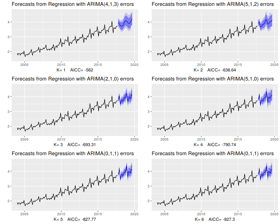
Figure 9.8: Using Fourier terms and ARIMA errors for forecasting monthly expenditure on eating out in Australia.