8.4 Moving average models

Rather than using past values of the forecast variable in a regression, a moving average model uses past forecast errors in a regression-like model. \[ y_{t} = c + e_t + \theta_{1}e_{t-1} + \theta_{2}e_{t-2} + \dots + \theta_{q}e_{t-q}, \] where $e_t$ is white noise. We refer to this as an MA($q$) model. Of course, we do not observe the values of $e_t$, so it is not really a regression in the usual sense.

Notice that each value of $y_t$ can be thought of as a weighted moving average of the past few forecast errors. However, moving average models should not be confused with the moving average smoothing we discussed in Chapter 6. A moving average model is used for forecasting future values, while moving average smoothing is used for estimating the trend-cycle of past values.

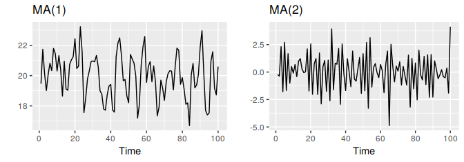
$Two examples of data from moving average models with different parameters. Left: MA(1) with $y_t = 20 + e_t + 0.8e_{t-1}$. Right: MA(2) with $y_t = e_t- e_{t-1}+0.8e_{t-2}$. In both cases, $e_t$ is normally distributed white noise with mean zero and variance one.$

Figure 8.6: Two examples of data from moving average models with different parameters. Left: MA(1) with $y_t = 20 + e_t + 0.8e_{t-1}$. Right: MA(2) with $y_t = e_t- e_{t-1}+0.8e_{t-2}$. In both cases, $e_t$ is normally distributed white noise with mean zero and variance one.

Figure 8.6 shows some data from an MA(1) model and an MA(2) model. Changing the parameters $\theta_1,\dots,\theta_q$ results in different time series patterns. As with autoregressive models, the variance of the error term $e_t$ will only change the scale of the series, not the patterns.

It is possible to write any stationary AR($p$) model as an MA($\infty$) model. For example, using repeated substitution, we can demonstrate this for an AR(1) model: \[\begin{align*} y_t &= \phi_1y_{t-1} + e_t\\ &= \phi_1(\phi_1y_{t-2} + e_{t-1}) + e_t\\ &= \phi_1^2y_{t-2} + \phi_1 e_{t-1} + e_t\\ &= \phi_1^3y_{t-3} + \phi_1^2e_{t-2} + \phi_1 e_{t-1} + e_t\\ &\text{etc.} \end{align*}\]

Provided $-1 < \phi_1 < 1$, the value of $\phi_1^k$ will get smaller as $k$ gets larger. So eventually we obtain \[ y_t = e_t + \phi_1 e_{t-1} + \phi_1^2 e_{t-2} + \phi_1^3 e_{t-3} + \cdots, \] an MA($\infty$) process.

The reverse result holds if we impose some constraints on the MA parameters. Then the MA model is called “invertible”. That is, we can write any invertible MA($q$) process as an AR($\infty$) process.

Invertible models are not simply introduced to enable us to convert from MA models to AR models. They also have some mathematical properties that make them easier to use in practice.

The invertibility constraints are similar to the stationarity constraints.

For an MA(1) model: $-1<\theta_1<1$.
For an MA(2) model: $-1<\theta_2<1$, $\theta_2+\theta_1 >-1$, $\theta_1 -\theta_2 < 1$.

More complicated conditions hold for $q\ge3$. Again, R will take care of these constraints when estimating the models.