12.4 Forecast combinations

An easy way to improve forecast accuracy is to use several different methods on the same time series, and to average the resulting forecasts. Nearly 50 years ago, John Bates and Clive Granger wrote a famous paper (Bates and Granger 1969), showing that combining forecasts often leads to better forecast accuracy. Twenty years later, Clemen (1989) wrote

The results have been virtually unanimous: combining multiple forecasts leads to increased forecast accuracy. in many cases one can make dramatic performance improvements by simply averaging the forecasts.

While there has been considerable research on using weighted averages, or some other more complicated combination approach, using a simple average has proven hard to beat.

Here is an example using monthly expenditure on eating out in Australia, from April 1982 to September 2017. We use forecast from the following models: ETS, ARIMA, STL-ETS, NNAR, and TBATS; and we compare the results using the last 5 years (60 months) of observations.

train <- window(auscafe, end=c(2012,9))
h <- length(auscafe) - length(train)
ETS <- forecast(ets(train), h=h)
ARIMA <- forecast(auto.arima(train, lambda=0, biasadj=TRUE), h=h)
STL <- stlf(train, lambda=0, h=h, biasadj=TRUE)
NNAR <- forecast(nnetar(train), h=h)
TBATS <- forecast(tbats(train), h=h)
Combination <- (ETS$mean + ARIMA$mean + STL$mean + NNAR$mean + TBATS$mean)/5

autoplot(auscafe) +
  forecast::autolayer(ETS$mean, series="ETS") +
  forecast::autolayer(ARIMA$mean, series="ARIMA") +
  forecast::autolayer(STL$mean, series="STL") +
  forecast::autolayer(STL$mean, series="NNAR") +
  forecast::autolayer(STL$mean, series="TBATS") +
  forecast::autolayer(Combination, series="Combination") +
  xlab("Year") + ylab("$ billion") +
  ggtitle("Australian monthly expenditure on eating out")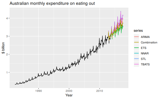

c(ETS=accuracy(ETS, auscafe)["Test set","RMSE"],
  ARIMA=accuracy(ARIMA, auscafe)["Test set","RMSE"],
  `STL-ETS`=accuracy(STL, auscafe)["Test set","RMSE"],
  NNAR=accuracy(NNAR, auscafe)["Test set","RMSE"],
  TBATS=accuracy(TBATS, auscafe)["Test set","RMSE"],
  Combination=accuracy(Combination, auscafe)["Test set","RMSE"])
#>         ETS       ARIMA     STL-ETS        NNAR       TBATS Combination 
#>      0.1370      0.1215      0.2145      0.3177      0.0884      0.0719

TBATS does particularly well with this series, but the combination approach is not far behind. For other data, TBATS may be quite poor, while the combination approach is almost always close to, or better than, the best component method.

References

Bates, J M, and C W J Granger. 1969. “The Combination of Forecasts.” Operational Research Quarterly 20 (4). Operational Research Society: 451–68. https://doi.org/10.1057/jors.1969.103.

Clemen, R. 1989. “Combining Forecasts: A Review and Annotated Bibliography with Discussion.” International Journal of Forecasting 5: 559–608.