6.1 Time series components

If we assume an additive model, then we can write \[ y_{t} = S_{t} + T_{t} + R_t, \] where \(y_{t}\) is the data at period \(t\), \(S_{t}\) is the seasonal component at period \(t\), \(T_{t}\) is the trend-cycle component at period \(t\) and \(R_t\) is the remainder component at period \(t\). Alternatively, a multiplicative model would be written as \[ y_{t} = S_{t} \times T_{t} \times R_t. \]

The additive model is the most appropriate if the magnitude of the seasonal fluctuations, or the variation around the trend-cycle, does not vary with the level of the time series. When the variation in the seasonal pattern, or the variation around the trend-cycle, appears to be proportional to the level of the time series, then a multiplicative model is more appropriate. Multiplicative models are common with economic time series.

An alternative to using a multiplicative model is to first transform the data until the variation in the series appears to be stable over time, then use an additive model. When a log transformation has been used, this is equivalent to using a multiplicative decomposition because \[ y_{t} = S_{t} \times T_{t} \times R_t \quad\text{is equivalent to}\quad \log y_{t} = \log S_{t} + \log T_{t} + \log R_t. \]

Electrical equipment manufacturing

We will look at several methods for obtaining the components \(S_{t}\), \(T_{t}\) and \(R_{t}\) later in this chapter, but first, it is helpful to see an example. We will decompose the new orders index for electrical equipment shown in Figure 6.1. These data show the numbers of new orders for electrical equipment (computer, electronic and optical products) in the Euro area (16 countries). The data have been adjusted by working days and normalized so that a value of 100 corresponds to 2005.

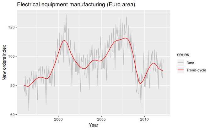
Figure 6.1: Electrical equipment orders: the trend-cycle component (red) and the raw data (grey).

Figure 6.1 shows the trend-cycle component, \(T_t\), in red and the original data, \(y_t\), in grey. The trend-cycle shows the overall movement in the series, ignoring the seasonality and any small random fluctuations.

Figure 6.2 shows an additive decomposition of these data. The method used for estimating components in this example is STL, which is discussed in Section 6.6.

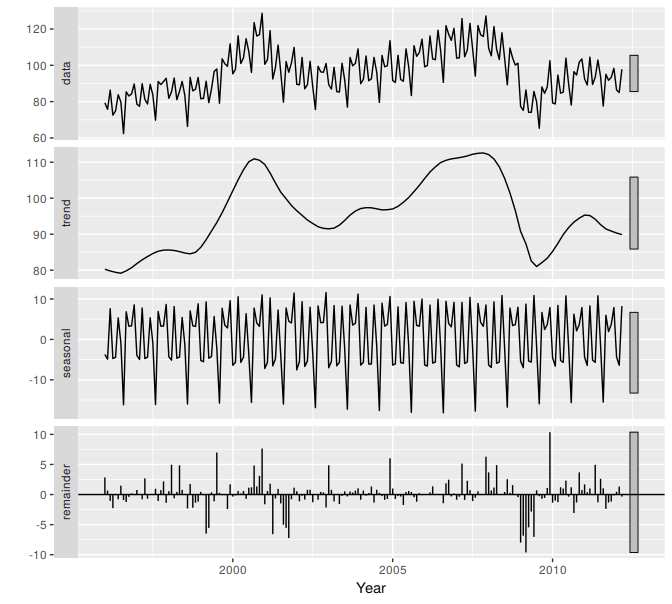
Figure 6.2: The electricial equipment orders (top) and its three additive components.

The three components are shown separately in the bottom three panels of Figure 6.2. These components can be added together to reconstruct the data shown in the top panel. Notice that the seasonal component changes very slowly over time, so that any two consecutive years have very similar patterns, but years far apart may have different seasonal patterns. The remainder component shown in the bottom panel is what is left over when the seasonal and trend-cycle components have been subtracted from the data.

The grey bars to the right of each panel show the relative scales of the components. Each grey bar represents the same length but because the plots are on different scales, the bars vary in size. The large grey bar in the bottom panel shows that the variation in the remainder component is small compared to the variation in the data, which has a bar about one quarter the size. If we shrunk the bottom three panels until their bars became the same size as that in the data panel, then all the panels would be on the same scale.

Seasonally adjusted data

If the seasonal component is removed from the original data, the resulting values are called the “seasonally adjusted” data. For an additive model, the seasonally adjusted data are given by \(y_{t}-S_{t}\), and for multiplicative data, the seasonally adjusted values are obtained using \(y_{t}/S_{t}\).

Figure 6.3 shows the seasonally adjusted electrical equipment orders.

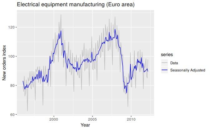
Figure 6.3: Seasonally adjusted electrical equipment orders (red) and the original data (grey).

If the variation due to seasonality is not of primary interest, the seasonally adjusted series can be useful. For example, monthly unemployment data are usually seasonally adjusted in order to highlight variation due to the underlying state of the economy rather than the seasonal variation. An increase in unemployment due to school leavers seeking work is seasonal variation, while an increase in unemployment due to large employers laying off workers is non-seasonal. Most people who study unemployment data are more interested in the non-seasonal variation. Consequently, employment data (and many other economic series) are usually seasonally adjusted.

Seasonally adjusted series contain the remainder component as well as the trend-cycle. Therefore, they are not “smooth”, and “downturns” or “upturns” can be misleading. If the purpose is to look for turning points in the series, and interpret any changes in the series, then it is better to use the trend-cycle component rather than the seasonally adjusted data.