9.2 Regression with ARIMA errors in R
The R function Arima() will fit a regression model with ARIMA errors if the argument xreg is used. The order argument specifies the order of the ARIMA error model. If differencing is specified, then the differencing is applied to all variables in the regression model before the model is estimated. For example, the R command
fit <- Arima(y, xreg=x, order=c(1,1,0))will fit the model \(y_t' = \beta_1 x'_t + n'_t\), where \(n'_t = \phi_1 n'_{t-1} + e_t\) is an AR(1) error. This is equivalent to the model
\[
y_t = \beta_0 + \beta_1 x_t + n_t,
\]
where \(n_t\) is an ARIMA(1,1,0) error. Notice that the constant term disappears
due to the differencing. To include a constant in the differenced
model, specify include.drift=TRUE.
The auto.arima() function will also handle regression terms via the xreg argument. The user must specify the predictor variables to include, but auto.arima will select the best ARIMA model for the errors.
The AICc is calculated for the final model, and this value can be used to determine the best predictors. That is, the procedure should be repeated for all subsets of predictors to be considered, and the model with the lowest AICc value selected.
Example: US Personal Consumption and Income
Figure 9.1 shows the quarterly changes in personal consumption expenditure and personal disposable income from 1970 to 2010. We would like to forecast changes in expenditure based on changes in income. A change in income does not necessarily translate to an instant change in consumption (e.g., after the loss of a job, it may take a few months for expenses to be reduced to allow for the new circumstances). However, we will ignore this complexity in this example and try to measure the instantaneous effect of the average change of income on the average change of consumption expenditure.
autoplot(uschange[,1:2], facets=TRUE) +
  xlab("Year") + ylab("") +
  ggtitle("Quarterly changes in US consumption and personal income")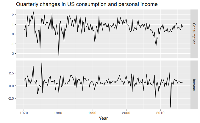
Figure 9.1: Percentage changes in quarterly personal consumption expenditure and personal disposable income for the USA, 1970 to 2010.
(fit <- auto.arima(uschange[,"Consumption"], xreg=uschange[,"Income"]))
#> Series: uschange[, "Consumption"]
#> Regression with ARIMA(1,0,2) errors
#>
#> Coefficients:
#>         ar1     ma1    ma2  intercept   xreg
#>       0.692  -0.576  0.198      0.599  0.203
#> s.e.  0.116   0.130  0.076      0.088  0.046
#>
#> sigma^2 estimated as 0.322:  log likelihood=-157
#> AIC=326   AICc=326   BIC=345
The data are clearly already stationary (as we are considering percentage changes rather than raw expenditure and income), so there is no need for any differencing. The fitted model is \[\begin{align*} y_t &= 0.60 + NA x_t + n_t, \\ n_t &= 0.69 n_{t-1} + e_t -0.58 e_{t-1} + 0.20 e_{t-2},\\ e_t &\sim \text{NID}(0,0.322). \end{align*}\]
We can recover both the \(n_t\) and \(e_t\) series using the residuals() function.
cbind("Regression Errors" = residuals(fit, type="regression"),
      "ARIMA errors" = residuals(fit, type="innovation")) %>%
  autoplot(facets=TRUE)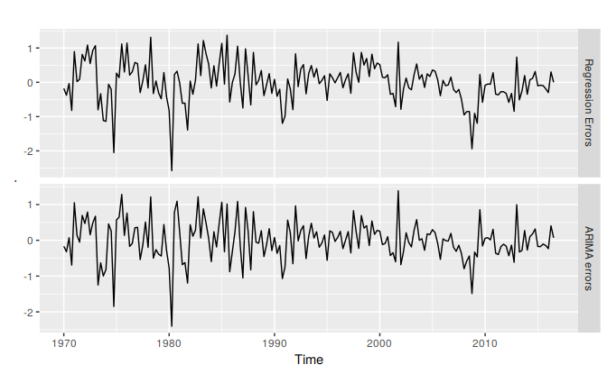
Figure 9.2: Regression errors (\(n_t\)) and ARIMA errors (\(e_t\)) from the fitted model.
It is the ARIMA errors that should resemble a white noise series.
checkresiduals(fit)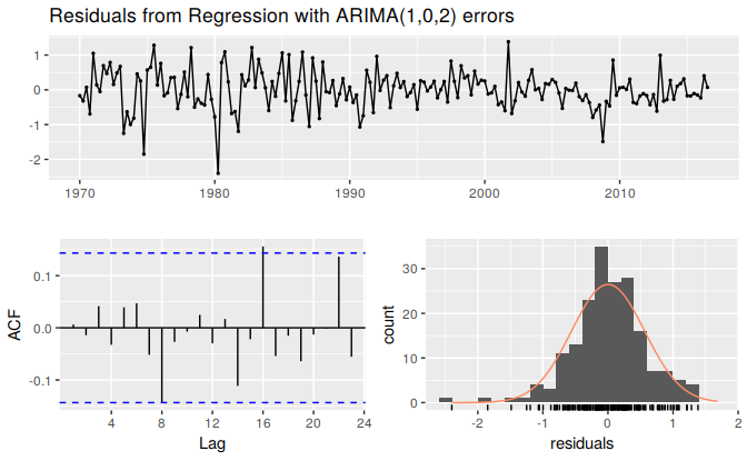
Figure 9.3: The residuals (i.e., the ARIMA errors) are not significantly different from white noise.
#>
#>  Ljung-Box test
#>
#> data:  Residuals from Regression with ARIMA(1,0,2) errors
#> Q* = 6, df = 3, p-value = 0.1
#>
#> Model df: 5.   Total lags used: 8