12.1 Weekly, daily and sub-daily data

Weekly, daily and sub-daily data can be challenging for forecasting, although for different reasons.

Weekly data

Weekly data is difficult because the seasonal period (the number of weeks in a year) is both large and non-integer. The average number of weeks in a year is 52.18. Most of the methods we have considered require the seasonal period to be an integer. Even if we approximate it by 52, most of the methods will not handle such a large seasonal period efficiently.

The simplest approach is to use a dynamic harmonic regression model, as discussed in Section 9.5. Here is an example using weekly data on US finished motor gasoline products supplied (in thousands of barrels per day) from February 1991 to May 2005. The number of Fourier terms was selected by minimizing the AICc. The order of the ARIMA model is also selected by minimizing the AICc, although that is done within the auto.arima() function.

bestfit <- list(aicc=Inf)
for(K in seq(25))
{
  fit <- auto.arima(gasoline, xreg=fourier(gasoline, K=K), seasonal=FALSE)
  if(fit$aicc < bestfit$aicc)
  {
    bestfit <- fit
    bestK <- K
  }
}
fc <- forecast(bestfit, xreg=fourier(gasoline, K=bestK, h=104))
autoplot(fc)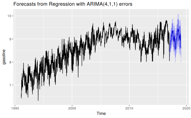

The fitted model has 18 pairs of Fourier terms and can be written as:

\[ y_t = bt + \sum_{j=1}^{18} \left[ \alpha_j\sin\left(\frac{2\pi j t}{52.18}\right) + \beta_j\cos\left(\frac{2\pi j t}{52.18}\right) \right] + n_t \] where \(n_t\) is an Regression with ARIMA(4,1,1) errors process. Because \(n_t\) is non-stationary, the model is actually estimated on the differences of the variables on both sides of this equation. There are 36 parameters to capture the seasonality which is rather a lot, but apparently required according to the AICc selection. The total number of degrees of freedom is 42 (the other three coming from the 2 MA parameters and the drift parameter).

An alternative approach is the TBATS model introduced in Section 11.1. This was the subject of Exercise 11.2. In this example, the forecasts are almost identical and there is little to differentiate the two models. The TBATS model is preferable when the seasonality changes over time. The ARIMA approach is preferable if there are covariates that are useful predictors as these can be added as additional regressors.

Daily and sub-daily data

Daily and sub-daily data are challenging for a different reason — they often involve multiple seasonal patterns, and so we need to use a method that handles such complex seasonality.

Of course, if the time series is relatively short so that only one type of seasonality is present, than it will be possible to use one of the single-seasonal methods we have discussed (e.g., ETS or seasonal ARIMA). But when the time series is long enough so that some of the longer seasonal periods become apparent, it will be necessary to use dynamic harmonic regression or TBATS, as discussed in Section 11.1.

However, note that even these models only allow for regular seasonality. Capturing seasonality associated with moving events such as Easter, Id, or the Chinese New Year is more difficult. Even with monthly data, this can be tricky as the festivals can fall in either March or April (for Easter), in January or February (for the Chinese New Year), or at any time of the year (for Id).

The best way to deal with moving holiday effects is to use dummy variables. However, neither ETS nor TBATS models allow for covariates. Amongst the models discussed in this book (and implemented in the forecast package for R), the only choice is a dynamic regression model, where the predictors include any dummy holiday effects (and possibly also the seasonality using Fourier terms).