7.2 Trend methods
###Holt’s linear trend method {-}
Holt (1957) extended simple exponential smoothing to allow the forecasting of data with a trend. This method involves a forecast equation and two smoothing equations (one for the level and one for the trend): \[\begin{align*} \text{Forecast equation}&& \hat{y}_{t+h|t} &= \ell_{t} + hb_{t} \\ \text{Level equation} && \ell_{t} &= \alpha y_{t} + (1 - \alpha)(\ell_{t-1} + b_{t-1})\\ \text{Trend equation} && b_{t} &= \beta^*(\ell_{t} - \ell_{t-1}) + (1 -\beta^*)b_{t-1}, \end{align*}\] where \(\ell_t\) denotes an estimate of the level of the series at time \(t\), \(b_t\) denotes an estimate of the trend (slope) of the series at time \(t\), \(\alpha\) is the smoothing parameter for the level, \(0\le\alpha\le1\), and \(\beta^*\) is the smoothing parameter for the trend, \(0\le\beta^*\le1\). (We denote this as \(\beta^*\) instead of \(\beta\) for reasons that will be explained in Section 7.5.)
As with simple exponential smoothing, the level equation here shows that \(\ell_t\) is a weighted average of observation \(y_t\) and the one-step-ahead training forecast for time \(t\), here given by \(\ell_{t-1} + b_{t-1}\). The trend equation shows that \(b_t\) is a weighted average of the estimated trend at time \(t\) based on \(\ell_{t} - \ell_{t-1}\) and \(b_{t-1}\), the previous estimate of the trend.
The forecast function is no longer flat but trending. The \(h\)-step-ahead forecast is equal to the last estimated level plus \(h\) times the last estimated trend value. Hence the forecasts are a linear function of \(h\).
Example: Air Passengers
air <- window(ausair, start=1990)
autoplot(air) +
 ggtitle("Air passengers in Australia") +
  xlab("Year") + ylab("millions of passengers")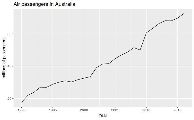
Figure 7.3: Total annual passengers of air carriers registered in Australia. 1990-2014.
Figure 7.3 shows annual passenger numbers for Australian airlines. In Table 7.3 we demonstrate the application of Holt’s method to these data. The smoothing parameters, \(\alpha\) and \(\beta\), and the initial values \(\ell_0\) and \(b_0\) are estimated by minimizing the SSE for the one-step training errors as in Section 7.1.
fc <- holt(air, h=5)| Year | Time | Observation | Level | Slope | Forecast |
|---|---|---|---|---|---|
| \(t\) | \(y_t\) | \(\ell_t\) | \(b_t\) | \(\hat{y}_{t|t-1}\) | |
| 1989 | 0 | 15.57 | 2.102 | ||
| 1990 | 1 | 17.55 | 17.57 | 2.102 | 17.67 |
| 1991 | 2 | 21.86 | 21.49 | 2.102 | 19.68 |
| 1992 | 3 | 23.89 | 23.84 | 2.102 | 23.59 |
| 1993 | 4 | 26.93 | 26.76 | 2.102 | 25.94 |
| 1994 | 5 | 26.89 | 27.22 | 2.102 | 28.86 |
| 1995 | 6 | 28.83 | 28.92 | 2.102 | 29.33 |
| 1996 | 7 | 30.08 | 30.24 | 2.102 | 31.02 |
| 1997 | 8 | 30.95 | 31.19 | 2.102 | 32.34 |
| 1998 | 9 | 30.19 | 30.71 | 2.101 | 33.29 |
| 1999 | 10 | 31.58 | 31.79 | 2.101 | 32.81 |
| 2000 | 11 | 32.58 | 32.80 | 2.101 | 33.89 |
| 2001 | 12 | 33.48 | 33.72 | 2.101 | 34.90 |
| 2002 | 13 | 39.02 | 38.48 | 2.101 | 35.82 |
| 2003 | 14 | 41.39 | 41.25 | 2.101 | 40.58 |
| 2004 | 15 | 41.60 | 41.89 | 2.101 | 43.35 |
| 2005 | 16 | 44.66 | 44.54 | 2.101 | 44.00 |
| 2006 | 17 | 46.95 | 46.90 | 2.101 | 46.65 |
| 2007 | 18 | 48.73 | 48.78 | 2.101 | 49.00 |
| 2008 | 19 | 51.49 | 51.38 | 2.101 | 50.88 |
| 2009 | 20 | 50.03 | 50.61 | 2.101 | 53.49 |
| 2010 | 21 | 60.64 | 59.30 | 2.102 | 52.72 |
| 2011 | 22 | 63.36 | 63.03 | 2.102 | 61.40 |
| 2012 | 23 | 66.36 | 66.15 | 2.102 | 65.13 |
| 2013 | 24 | 68.20 | 68.21 | 2.102 | 68.25 |
| 2014 | 25 | 68.12 | 68.49 | 2.102 | 70.31 |
| 2015 | 26 | 69.78 | 69.92 | 2.102 | 70.60 |
| 2016 | 27 | 72.60 | 72.50 | 2.102 | 72.02 |
| \(h\) | \(\hat{y}_{t+h|t}\) | ||||
| 1 | 74.60 | ||||
| 2 | 76.70 | ||||
| 3 | 78.80 | ||||
| 4 | 80.91 | ||||
| 5 | 83.01 |
The very small value of \(\beta^*\) means that the slope hardly changes over time. Figure 7.4 shows the forecasts for years 2014–2018.
Damped trend methods
The forecasts generated by Holt’s linear method display a constant trend (increasing or decreasing) indefinitely into the future. Empirical evidence indicates that these methods tend to over-forecast, especially for longer forecast horizons. Motivated by this observation, Gardner Jr and McKenzie (1985) introduced a parameter that “dampens” the trend to a flat line some time in the future. Methods that include a damped trend have proven to be very successful, and are arguably the most popular individual methods when forecasts are required automatically for many series.
In conjunction with the smoothing parameters \(\alpha\) and \(\beta^*\) (with values between 0 and 1 as in Holt’s method), this method also includes a damping parameter \(0<\phi<1\): \[\begin{align*} \hat{y}_{t+h|t} &= \ell_{t} + (\phi+\phi^2 + \dots + \phi^{h})b_{t} \\ \ell_{t} &= \alpha y_{t} + (1 - \alpha)(\ell_{t-1} + \phi b_{t-1})\\ b_{t} &= \beta^*(\ell_{t} - \ell_{t-1}) + (1 -\beta^*)\phi b_{t-1}. \end{align*}\] If \(\phi=1\), the method is identical to Holt’s linear method. For values between \(0\) and \(1\), \(\phi\) dampens the trend so that it approaches a constant some time in the future. In fact, the forecasts converge to \(\ell_T+\phi b_T/(1-\phi)\) as \(h\rightarrow\infty\) for any value \(0<\phi<1\). This means that short-run forecasts are trended while long-run forecasts are constant.
In practice, \(\phi\) is rarely less than 0.8 as the damping has a very strong effect for smaller values. Values of \(\phi\) close to 1 will mean that a damped model is not able to be distinguished from a non-damped model. For these reasons, we usually restrict \(\phi\) to a minimum of 0.8 and a maximum of 0.98.
Example: Air Passengers (continued)
Figure 7.4 shows the forecasts for years 2014–2018 generated from Holt’s linear trend method and the damped trend method.
fc <- holt(air, h=15)
fc2 <- holt(air, damped=TRUE, phi = 0.9, h=15)
autoplot(air) +
  forecast::autolayer(fc$mean, series="Holt's method") +
  forecast::autolayer(fc2$mean, series="Damped Holt's method") +
  ggtitle("Forecasts from Holt's method") +
  xlab("Year") + ylab("Air passengers in Australia (millions)") +
  guides(colour=guide_legend(title="Forecast"))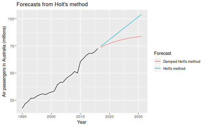
Figure 7.4: Forecasting Air Passengers in Australia (millions of passengers). For the damped trend method, \(\phi=0.90\).
We have set the damping parameter to a relatively low number \((\phi=0.90)\) to exaggerate the effect of damping for comparison. Usually, we would estimate \(\phi\) along with the other parameters.
Example: Sheep in Asia
In this example, we compare the forecasting performance of the three exponential smoothing methods that we have considered so far in forecasting the sheep livestock population in Asia. The data spans the period 1970–2007 and is shown in Figure 7.5.
autoplot(livestock) +
  xlab("Year") + ylab("Livestock, sheep in Asia (millions)")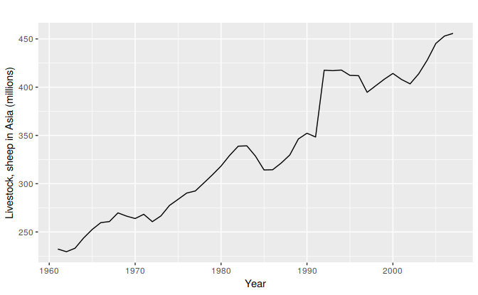
Figure 7.5: Annual sheep livestock numbers in Asia (in million head)
We will use time series cross-validation to compare the one-step forecast accuracy of the three methods.
e1 <- tsCV(livestock, ses, h=1)
e2 <- tsCV(livestock, holt, h=1)
e3 <- tsCV(livestock, holt, damped=TRUE, h=1)
# Compare MSE:
mean(e1^2, na.rm=TRUE)
#> [1] 178
mean(e2^2, na.rm=TRUE)
#> [1] 173
mean(e3^2, na.rm=TRUE)
#> [1] 163
# Compare MAE:
mean(abs(e1), na.rm=TRUE)
#> [1] 8.53
mean(abs(e2), na.rm=TRUE)
#> [1] 8.8
mean(abs(e3), na.rm=TRUE)
#> [1] 8.02
Based on MSE, Holt’s method is best. But based on MAE, simple exponential smoothing is best. Conflicts such as this are common in forecasting comparisons. As forecasting tasks can vary by many dimensions (length of forecast horizon, size of test set, forecast error measures, frequency of data, etc.), it is unlikely that one method will be better than all others for all forecasting scenarios. What we require from a forecasting method are consistently sensible forecasts, and these should be frequently evaluated against the task at hand. In this case, the data are clearly trended, so we will prefer Holt’s method, and apply it to the whole data set to get forecasts for future years.
fc <- holt(livestock)
# Estimated parameters:
fc[["model"]]
#> Holt's method
#>
#> Call:
#>  holt(y = livestock)
#>
#>   Smoothing parameters:
#>     alpha = 0.9999
#>     beta  = 1e-04
#>
#>   Initial states:
#>     l = 225.4909
#>     b = 4.9513
#>
#>   sigma:  12.6
#>
#>  AIC AICc  BIC
#>  425  426  434
The smoothing parameter for the slope parameter is estimated to be essentially zero, indicating that the trend is not changing over time. The value of \(\alpha\) is very close to one, showing that the level reacts strongly to each new observation.
autoplot(fc) +
  xlab("Year") + ylab("Livestock, sheep in Asia (millions)")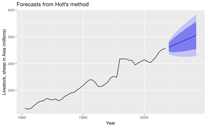
Figure 7.6: Forecasting livestock, sheep in Asia: comparing forecasting performance of non-seasonal method.
The resulting forecasts look sensible with increasing trend, and relatively wide prediction intervals reflecting the variation in the historical data. The prediction intervals are calculated using the methods described in Section 7.5.
References
Gardner Jr, Everette S, and Ed McKenzie. 1985. “Forecasting Trends in Time Series.” Management Science 31 (10): 1237–46.
Holt, Charles E. 1957. “Forecasting Seasonals and Trends by Exponentially Weighted Averages.” O.N.R. Memorandum 52. Carnegie Institute of Technology, Pittsburgh USA.