3.2 Transformations and adjustments
Adjusting the historical data can often lead to a simpler forecasting model. Here, we deal with four kinds of adjustments: calendar adjustments, population adjustments, inflation adjustments and mathematical transformations. The purpose of these adjustments and transformations is to simplify the patterns in the historical data by removing known sources of variation or by making the pattern more consistent across the whole data set. Simpler patterns usually lead to more accurate forecasts.
Calendar adjustments
Some of the variation seen in seasonal data may be due to simple calendar effects. In such cases, it is usually much easier to remove the variation before fitting a forecasting model. The monthdays function will compute the number of days in each month or quarter.
For example, if you are studying the monthly milk production on a farm, there will be variation between the months simply because of the different numbers of days in each month, in addition to the seasonal variation across the year.
dframe <- cbind(Monthly = milk, DailyAverage=milk/monthdays(milk))
  autoplot(dframe, facet=TRUE) + xlab("Years") + ylab("Pounds") +
    ggtitle("Milk production per cow")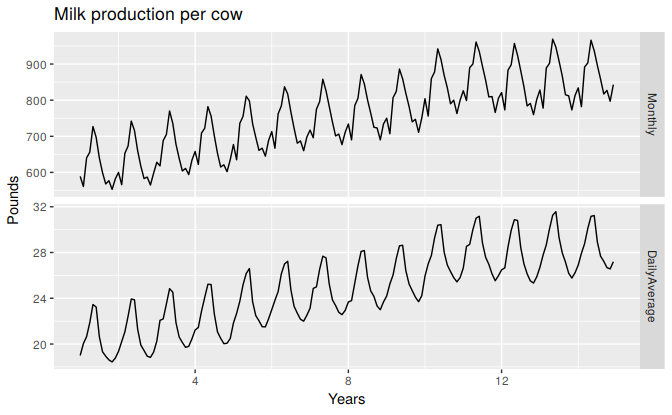
Figure 3.3: Monthly milk production per cow. Source: Cryer and Chan (2008).
Notice how much simpler the seasonal pattern is in the average daily production plot compared to the average monthly production plot. By looking at the average daily production instead of the average monthly production, we effectively remove the variation due to the different month lengths. Simpler patterns are usually easier to model and lead to more accurate forecasts.
A similar adjustment can be done for sales data when the number of trading days in each month varies. In this case, the sales per trading day can be modelled instead of the total sales for each month.
Population adjustments
Any data that are affected by population changes can be adjusted to give per-capita data. That is, consider the data per person (or per thousand people, or per million people) rather than the total. For example, if you are studying the number of hospital beds in a particular region over time, the results are much easier to interpret if you remove the effects of population changes by considering the number of beds per thousand people. Then you can see whether there have been real increases in the number of beds, or whether the increases are due entirely to population increases. It is possible for the total number of beds to increase, but the number of beds per thousand people to decrease. This occurs when the population is increasing faster than the number of hospital beds. For most data that are affected by population changes, it is best to use per-capita data rather than the totals.
Inflation adjustments
Data which are affected by the value of money are best adjusted before modelling. For example, the average cost of a new house will have increased over the last few decades due to inflation. A $200,000 house this year is not the same as a $200,000 house twenty years ago. For this reason, financial time series are usually adjusted so that all values are stated in dollar values from a particular year. For example, the house price data may be stated in year 2000 dollars.
To make these adjustments, a price index is used. If \(z_{t}\) denotes the price index and \(y_{t}\) denotes the original house price in year \(t\), then \(x_{t} = y_{t}/z_{t} * z_{2000}\) gives the adjusted house price at year 2000 dollar values. Price indexes are often constructed by government agencies. For consumer goods, a common price index is the Consumer Price Index (or CPI).
Mathematical transformations
If the data show variation that increases or decreases with the level of the series, then a transformation can be useful. For example, a logarithmic transformation is often useful. If we denote the original observations as \(y_{1},\dots,y_{T}\) and the transformed observations as \(w_{1}, \dots, w_{T}\), then \(w_t = \log(y_t)\). Logarithms are useful because they are interpretable: changes in a log value are relative (or percentage) changes on the original scale. So if log base 10 is used, then an increase of 1 on the log scale corresponds to a multiplication of 10 on the original scale. Another useful feature of log transformations is that they constrain the forecasts to stay positive on the original scale.
Sometimes other transformations are also used (although they are not so interpretable). For example, square roots and cube roots can be used. These are called power transformations because they can be written in the form \(w_{t} = y_{t}^p\).
A useful family of transformations, that includes both logarithms and power transformations, is the family of “Box-Cox transformations”, which depend on the parameter \(\lambda\) and are defined as follows: \[ w_t = \begin{cases} \log(y_t) & \text{if $\lambda=0$}; \\ (y_t^\lambda-1)/\lambda & \text{otherwise}. \end{cases} \]
The logarithm in a Box-Cox transformation is always a natural logarithm (i.e., to base \(e\)). So if \(\lambda=0\), natural logarithms are used, but if \(\lambda\ne0\), a power transformation is used, followed by some simple scaling.
If \(\lambda=1\), then \(w_t = y_t-1\), so the transformed data is shifted downwards but there is no change in the shape of the time series. But for all other values of \(\lambda\), the time series will change shape.
Use the slider below to see the effect of varying \(\lambda\) to transform Australian monthly electricity demand:
A good value of \(\lambda\) is one which makes the size of the seasonal variation about the same across the whole series, as that makes the forecasting model simpler. In this case, \(\lambda=0.30\) works quite well, although any value of \(\lambda\) between 0 and 0.5 would give similar results.
The BoxCox.lambda() function will choose a value of lambda for you.
(lambda <- BoxCox.lambda(elec))
#> [1] 0.265
autoplot(BoxCox(elec,lambda))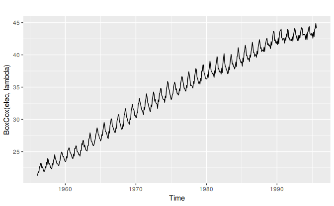
Having chosen a transformation, we need to forecast the transformed data. Then, we need to reverse the transformation (or back-transform) to obtain forecasts on the original scale. The reverse Box-Cox transformation is given by \[\begin{equation} \tag{3.1} y_{t} = \begin{cases} \exp(w_{t}) & \text{if $\lambda=0$};\\ (\lambda w_t+1)^{1/\lambda} & \text{otherwise}. \end{cases} \end{equation}\]
Features of power transformations
- If some \(y_{t}\le0\), no power transformation is possible unless all observations are adjusted by adding a constant to all values.
- Choose a simple value of \(\lambda\). It makes explanations easier.
- The forecasting results are relatively insensitive to the value of \(\lambda\).
- Often no transformation is needed.
- Transformations sometimes make little difference to the forecasts but have a large effect on prediction intervals.
Bias adjustments
One issue with using mathematical transformations such as Box-Cox transformations is that the back-transformed forecast will not be the mean of the forecast distribution. In fact, it will usually be the median of the forecast distribution (assuming that the distribution on the transformed space is symmetric). For many purposes, this is acceptable, but occasionally the mean forecast is required. For example, you may wish to add up sales forecasts from various regions to form a forecast for the whole country. But medians do not add up, whereas means do.
For a Box-Cox transformation, the backtransformed mean is given by \[\begin{equation} \tag{3.2} y_t = \begin{cases} \exp(w_t)\left[1 + \frac{\sigma_h^2}{2}\right] & \text{if $\lambda=0$;}\\ (\lambda w_t+1)^{1/\lambda}\left[1 + \frac{\sigma_h^2(1-\lambda)}{2(\lambda w_t+1)^{2}}\right] & \text{otherwise;} \end{cases} \end{equation}\] where \(\sigma_h^2\) is the \(h\)-step forecast variance. The larger the forecast variance, the bigger the difference between the mean and the median.
The difference between the simple back-transformed forecast given by (3.1) and the mean given by (3.2) is called the “bias”. When we use the mean, rather than the median, we say the point forecasts have been “bias-adjusted”. To see how much difference this bias-adjustment makes, consider the following example. Here we are forecasting the average annual price of eggs using the drift method with a log transformation \((\lambda=0)\). The log transformation is useful in this case to ensure the forecasts and the prediction intervals stay positive.
fc <- rwf(eggs, drift=TRUE, lambda=0, h=50, level=80)
fc2 <- rwf(eggs, drift=TRUE, lambda=0, h=50, level=80, biasadj=TRUE)
# autoplot(eggs) +
#   forecast::autolayer(fc, series="Simple back transformation") +
#   forecast::autolayer(fc2$mean, series="Bias adjusted") +
#   guides(colour=guide_legend(title="Forecast"))
The blue line shows the forecast medians while the red line shows the forecast means. Notice how the skewed forecast distribution pulls up the point forecast when we use the bias adjustment.
Bias adjustment is not done by default in the forecast package. If you want your forecasts to be means rather than medians, use the argument biadadj=TRUE when you select your Box-Cox transformation parameter.
References
Cryer, Jonathan D, and Kung-Sik Chan. 2008. Time Series Analysis: With Applications in R. Springer Texts in Statistics. New York: Springer.