2.2 Time plots
For time series data, the obvious graph to start with is a time plot. That is, the observations are plotted against the time of observation, with consecutive observations joined by straight lines. Figure 2.1 below shows the weekly economy passenger load on Ansett Airlines between Australia’s two largest cities.
autoplot(melsyd[,"Economy.Class"]) +
  ggtitle("Economy class passengers: Melbourne-Sydney") +
  xlab("Year") + ylab("Thousands")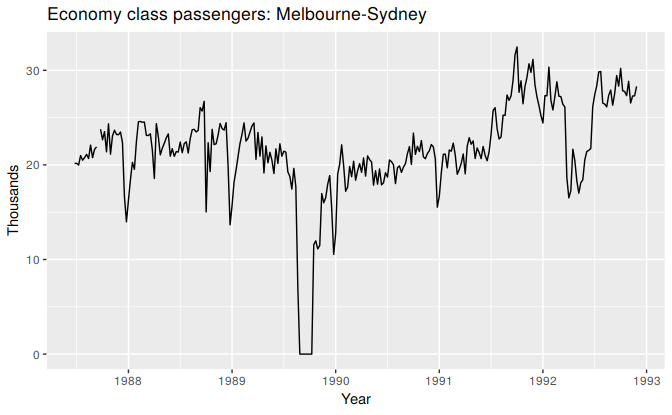
Figure 2.1: Weekly economy passenger load on Ansett Airlines.
We will use the autoplot command frequently. It automatically produces an appropriate plot of whatever you pass to it in the first argument. In this case, it recognizes melsyd[,"Economy.Class"] as a time series and produces a time plot.
The time plot immediately reveals some interesting features.
- There was a period in 1989 when no passengers were carried — this was due to an industrial dispute.
- There was a period of reduced load in 1992. This was due to a trial in which some economy class seats were replaced by business class seats.
- A large increase in passenger load occurred in the second half of 1991.
- There are some large dips in load around the start of each year. These are due to holiday effects.
- There is a long-term fluctuation in the level of the series which increases during 1987, decreases in 1989, and increases again through 1990 and 1991.
- There are some periods of missing observations.
Any model will need to take all these features into account in order to effectively forecast the passenger load into the future.
A simpler time series is shown in Figure 2.2.
autoplot(a10) +
  ggtitle("Antidiabetic drug sales") +
  ylab("$ million") + xlab("Year")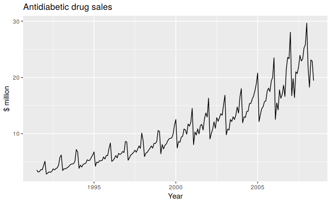
Figure 2.2: Monthly sales of antidiabetic drugs in Australia.
Here, there is a clear and increasing trend. There is also a strong seasonal pattern that increases in size as the level of the series increases. The sudden drop at the start of each year is caused by a government subsidisation scheme that makes it cost-effective for patients to stockpile drugs at the end of the calendar year.
Any forecasts of this series would need to capture the seasonal pattern, and the fact that the trend is changing slowly.