7.7 Forecasting with ETS models
Point forecasts are obtained from the models by iterating the equations for \(t=T+1,\dots,T+h\) and setting all \(\varepsilon_t=0\) for \(t>T\).
For example, for model ETS(M,A,N), \(y_{T+1} = (\ell_T + b_T )(1+ \varepsilon_{T+1}).\) Therefore \(\hat{y}_{T+1|T}=\ell_{T}+b_{T}.\) Similarly, \[\begin{align*} y_{T+2} &= (\ell_{T+1} + b_{T+1})(1 + \varepsilon_{T+1})\\ &= \left[ (\ell_T + b_T) (1+ \alpha\varepsilon_{T+1}) + b_T + \beta (\ell_T + b_T)\varepsilon_{T+1} \right] ( 1 + \varepsilon_{T+1}). \end{align*}\] Therefore, \(\hat{y}_{T+2|T}= \ell_{T}+2b_{T},\) and so on. These forecasts are identical to the forecasts from Holt’s linear method, and also to those from model ETS(A,A,N). Thus, the point forecasts obtained from the method and from the two models that underlie the method are identical (assuming that the same parameter values are used).
ETS point forecasts are equal to the medians of the forecast distributions. For models with only additive components, the forecast distributions are normal, so the medians and means are equal. For ETS models with multiplicative errors, or with multiplicative seasonality, the point forecasts will not be equal to the means of the forecast distributions.
To obtain forecasts from an ETS model, we use the forecast function. The R code below shows the possible arguments that this function takes when applied to an ETS model. We explain each of the arguments in what follows.
forecast(object, h=ifelse(object$m>1, 2*object$m, 10),
level=c(80,95), fan=FALSE, simulate=FALSE, bootstrap=FALSE, npaths=5000,
PI=TRUE, lambda=object$lambda, biasadj=NULL, ...)object- The object returned by the
ets()function. h- The forecast horizon — the number of periods to be forecast.
level- The confidence level for the prediction intervals.
fan- If
fan=TRUE,level=seq(50,99,by=1). This is suitable for fan plots. simulate- If
simulate=TRUE, prediction intervals are produced by simulation rather than using algebraic formulae. Simulation will also be used (even ifsimulate=FALSE) where there are no algebraic formulae available for the particular model. bootstrap- If
bootstrap=TRUEandsimulate=TRUE, then the simulated prediction intervals use re-sampled errors rather than normally distributed errors. npaths- The number of sample paths used in computing simulated prediction intervals.
PI- If
PI=TRUE, then prediction intervals are produced; otherwise only point forecasts are calculated. lambda- The Box-Cox transformation parameter. This is ignored if
lambda=NULL. Otherwise, the forecasts are back-transformed via an inverse Box-Cox transformation. biasadj- If
lambdais notNULL, the backtransformed forecasts (and prediction intervals) are bias-adjusted.
fit %>% forecast(h=8) %>%
  autoplot() +
  ylab("International visitor night in Australia (millions)")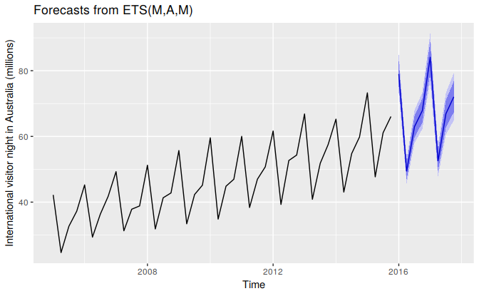
Figure 7.11: Forecasting international visitor nights in Australia using an ETS(M,A,M) model.
Prediction intervals
A big advantage of the models is that prediction intervals can also be generated — something that cannot be done using the methods. The prediction intervals will differ between models with additive and multiplicative methods.
For most ETS models, a prediction interval can be written as \[ \hat{y}_{T+h|T} \pm k \sigma_h \] where \(k\) depends on the coverage probability, and \(\sigma_h\) is the forecast variance. Values for \(k\) were given in Table 3.1. For ETS models, formulas for \(\sigma_h\) can be complicated; the details are given in Chapter 6 of Rob J Hyndman et al. (2008). In the table below, we give the formulas for the additive ETS models, which are the simplest.
Table: (#tab:pitable)Forecast variance expressions for each additive state space model, where \(\sigma^2\) is the residual variance, \(m\) is the seasonal period, \(h_m = \lfloor(h-1)/m\rfloor\) and \(\lfloor u\rfloor\) denotes the integer part of \(u\).
Model            Forecast variance: $\sigma_h$
---------------  -------------------------------------------------------------
(A,N,N)     $\sigma_h = \sigma^2\big[1 + \alpha^2(h-1)\big]$
(A,A,N)          $\sigma_h = \sigma^2\Big[1 + (h-1)\big\{\alpha^2 + \alpha\beta h + \frac16\beta^2h(2h-1)\big\}\Big]$
(A,A\damped,N)   $\sigma_h = \sigma^2\biggl[1 + \alpha^2(h-1) + \frac{\beta\phi h}{(1-\phi)^2} \left\{2\alpha(1-\phi) +\beta\phi\right\} - \frac{\beta\phi(1-\phi^h)}{(1-\phi)^2(1-\phi^2)} \left\{ 2\alpha(1-\phi^2)+ \beta\phi(1+2\phi-\phi^h)\right\}\biggr]$
(A,N,A)          $\sigma_h = \sigma^2\Big[1 + \alpha^2(h-1) + \gamma h_m(2\alpha+\gamma)\Big]$
(A,A,A)          $\sigma_h = \sigma^2\Big[1 + (h-1)\big\{\alpha^2 + \alpha\beta h + \frac16\beta^2h(2h-1)\big\} + \gamma h_m \big\{2\alpha+ \gamma + \beta m (h_m+1)\big\} \Big]$
(A,A\damped,A)   $\sigma_h = \sigma^2\biggl[1 + \alpha^2(h-1) +\frac{\beta\phi h}{(1-\phi)^2} \left\{2\alpha(1-\phi)  + \beta\phi \right\} - \frac{\beta\phi(1-\phi^h)}{(1-\phi)^2(1-\phi^2)} \left\{ 2\alpha(1-\phi^2)+ \beta\phi(1+2\phi-\phi^h)\right\}$
                                   ${} + \gamma h_m(2\alpha+\gamma)  + \frac{2\beta\gamma\phi}{(1-\phi)(1-\phi^m)}\left\{h_m(1-\phi^m) - \phi^m(1-\phi^{mh_m})\right\}\biggr]$
For a few ETS models, there are no known formulas for prediction intervals. In these cases, the forecast.ets function uses simulated future sample paths and computes prediction intervals from the percentiles of these simulated future paths.
Bagged ETS forecasts
A useful way to improve forecast accuracy is to generate multiple versions of the time series with slight variations. Then forecast from each of these additional time series, and average the resulting forecasts. This is called “bagging” which stands for “bootstrap aggregating”. The additional time series are bootstrapped versions of the original series, and we aggregate the results to get a better forecast.
We can combine STL decomposition and ETS model to get bagged ETS forecasts. First, the time series is Box-Cox-transformed, and then decomposed into trend, seasonal and remainder components using STL. Then we obtain shuffled versions of the remainder component to get bootstrapped remainder series. Because there may be autocorrelation present in an STL remainder series, we cannot simply use the re-draw procedure that was described in Section 3.5. Instead, we use a “blocked bootstrap”, where contiguous sections of the time series are selected at random and joined together. These bootstrapped remainder series are added to the trend and seasonal components, and the Box-Cox transformation is reversed to give variations on the original time series. Some examples are shown below for the Australian international tourist data.
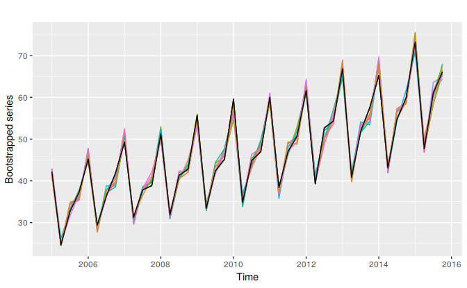
Figure 7.12: Ten bootstrapped versions of quarterly Australian tourist arrivals.
The coloured lines show ten bootstrapped series, while the black line is the original data. We use ets to forecast each of these series; it may choose a different model in each case, although most likely it will use the same model because the series are very similar. However, the parameters of the models will be different because the data are different. Consequently the forecast will vary also. Figure 7.13 shows the ten forecasts obtained in this way.
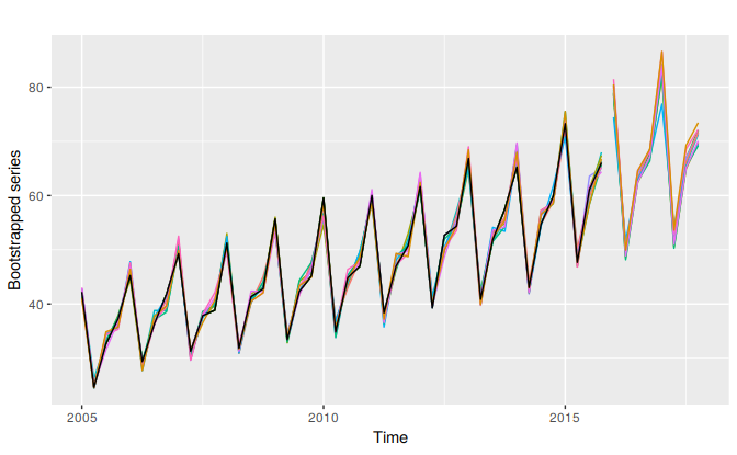
Figure 7.13: Forecasts of the ten bootstrapped series obtained using ETS models.
The average of these forecast gives the bagged forecasts of the original data. The whole procedure can be handled with the baggedETS function:
etsfc <- aust %>%
  ets %>% forecast(h=12)
baggedfc <- aust %>%
  baggedETS %>% forecast(h=12)
autoplot(aust) +
  forecast::autolayer(baggedfc$mean, series="BaggedETS") +
  forecast::autolayer(etsfc$mean, series="ETS") +
  guides(colour=guide_legend(title="Forecasts"))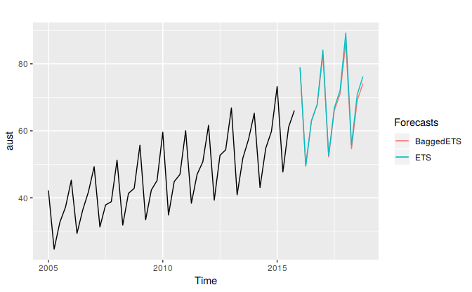
Figure 7.14: Comparing bagged ETS forecasts (the average of 100 bootstrapped forecast) and ETS applied directly to the data.
By default, 100 bootstrapped series are used, and the length of the blocks used for obtaining bootstrapped residuals is set to 8 for quarterly data.
In this case, it makes very little difference. Bergmeir, Hyndman, and Benıtez (2016) show that, on average, it gives better forecasts than just applying ets directly. Of course, it is slower because a lot more computation is required.
References
Bergmeir, Christoph, Rob J Hyndman, and José M Benıtez. 2016. “Bagging Exponential Smoothing Methods Using STL Decomposition and Box-Cox Transformation.” International Journal of Forecasting 32 (2): 303–12.
Hyndman, Rob J, Anne B Koehler, J Keith Ord, and Ralph D Snyder. 2008. Forecasting with Exponential Smoothing: The State Space Approach. Berlin: Springer-Verlag. www.exponentialsmoothing.net.