12.9 One-step forecasts on test data

It is common practice to fit a model using training data, and then to evaluate its performance on a test data set. The way this is usually done means the comparisions on the test data use different forecast horizons. For example, suppose we use the last twenty observations for the test data, and estimate our forecasting model on the training data. Then the forecast errors will be for 1-step, 2-steps, …, 20-steps ahead. The forecast variance usually increases with the forecast horizon, so if we simply averaging the absolute or squared errors from the test set, we are combining results with different variances.

One solution to this issue is to obtain 1-step errors on the test data. That is, we still use the training data to estimate any parameters, but when we compute forecasts on the test data, we use all of the data preceding each observation (both training and test data). To be specific, suppose our training data are for times \(1,2,\dots,T-20\). We estimate the model on these data, but then compute \(\hat{y}_{T-20+h|T-21+h}\), for \(h=1,\dots,T-1\). Because the test data are not used to estimate the parameters, this still gives us a “fair” forecast. For the ets, Arima, tbats and nnetar functions, these calculations are easily carried out using the model argument.

In the following example, we apply an ARIMA model to the Australian “eating out” monthly expenditure. The last five years are used as the test set.

training <- subset(auscafe, end=length(auscafe)-61)
test <- subset(auscafe, start=length(auscafe)-60)
cafe.train <- Arima(training, order=c(2,1,1), seasonal=c(0,1,2), lambda=0)
cafe.train %>% 
  forecast(h=60) %>% 
  autoplot() + forecast::autolayer(test)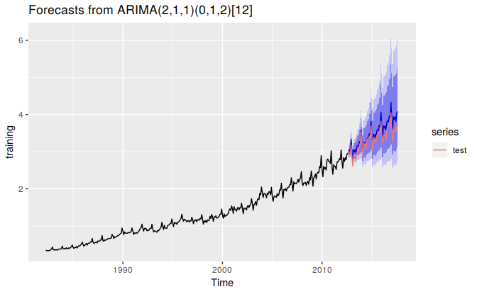

Now we apply the same model to the test data.

cafe.test <- Arima(test, model=cafe.train)
accuracy(cafe.test)
#>                    ME   RMSE    MAE    MPE MAPE MASE   ACF1
#> Training set -0.00262 0.0459 0.0341 -0.073    1 0.19 -0.057

Note that the second call to Arima does not involve the model being re-estimated. Instead, the model obtained in the first call is applied to the test data in the second call.

Because the model was not re-estimated, the “residuals” obtained here are actually one-step forecast errors. Consequently, the results produced from the accuracy command are actually on the test set (despite the output saying “Training set”).