1.4 Forecasting data and methods
The appropriate forecasting methods depend largely on what data are available.
If there are no data available, or if the data available are not relevant to the forecasts, then qualitative forecasting methods must be used. These methods are not purely guesswork—there are well-developed structured approaches to obtaining good forecasts without using historical data. These methods are discussed in Chapter 4.
Quantitative forecasting can be applied when two conditions are satisfied:
- numerical information about the past is available;
- it is reasonable to assume that some aspects of the past patterns will continue into the future.
There is a wide range of quantitative forecasting methods, often developed within specific disciplines for specific purposes. Each method has its own properties, accuracies, and costs that must be considered when choosing a specific method.
Most quantitative prediction problems use either time series data (collected at regular intervals over time) or cross-sectional data (collected at a single point in time). In this book we are concerned with forecasting future data, and we concentrate on the time series domain.
Time series forecasting
Examples of time series data include:
- Daily IBM stock prices
- Monthly rainfall
- Quarterly sales results for Amazon
- Annual Google profits
Anything that is observed sequentially over time is a time series. In this book, we will only consider time series that are observed at regular intervals of time (e.g., hourly, daily, weekly, monthly, quarterly, annually). Irregularly spaced time series can also occur, but are beyond the scope of this book.
When forecasting time series data, the aim is to estimate how the sequence of observations will continue into the future. Figure 1.1 shows the quarterly Australian beer production from 1992 to the second quarter of 2010.
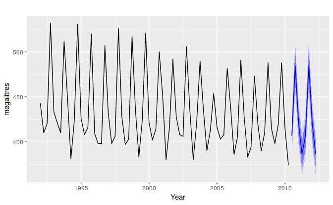
Figure 1.1: Australian quarterly beer production: 1992Q1–2010Q2, with two years of forecasts.
The blue lines show forecasts for the next two years. Notice how the forecasts have captured the seasonal pattern seen in the historical data and replicated it for the next two years. The dark shaded region shows 80% prediction intervals. That is, each future value is expected to lie in the dark shaded region with a probability of 80%. The light shaded region shows 95% prediction intervals. These prediction intervals are a very useful way of displaying the uncertainty in forecasts. In this case the forecasts are expected to be very accurate, and hence the prediction intervals are quite narrow.
The simplest time series forecasting methods use only information on the variable to be forecast, and make no attempt to discover the factors that affect its behaviour. Therefore they will extrapolate trend and seasonal patterns, but they ignore all other information such as marketing initiatives, competitor activity, changes in economic conditions, and so on.
Time series models used for forecasting include ARIMA models, exponential smoothing and structural models. These models are discussed in Chapters 6, 7 and 8.
Predictor variables and time series forecasting
Predictor variables can also be used in time series forecasting. For example, suppose we wish to forecast the hourly electricity demand (ED) of a hot region during the summer period. A model with predictor variables might be of the form \[\begin{align*} \text{ED} = & f(\text{current temperature, strength of economy, population,}\\ & \qquad\text{time of day, day of week, error}). \end{align*}\] The relationship is not exact—there will always be changes in electricity demand that cannot be accounted for by the predictor variables. The “error” term on the right allows for random variation and the effects of relevant variables that are not included in the model. We call this an “explanatory model” because it helps explain what causes the variation in electricity demand.
Because the electricity demand data form a time series, we could also use a time series model for forecasting. In this case, a suitable time series forecasting equation is of the form \[ \text{ED}_{t+1} = f(\text{ED}_{t}, \text{ED}_{t-1}, \text{ED}_{t-2}, \text{ED}_{t-3},\dots, \text{error}), \] where \(t\) is the present hour, \(t+1\) is the next hour, \(t-1\) is the previous hour, \(t-2\) is two hours ago, and so on. Here, prediction of the future is based on past values of a variable, but not on external variables which may affect the system. Again, the “error” term on the right allows for random variation and the effects of relevant variables that are not included in the model.
There is also a third type of model which combines the features of the above two models. For example, it might be given by \[ \text{ED}_{t+1} = f(\text{ED}_{t}, \text{current temperature, time of day, day of week, error}). \] These types of mixed models have been given various names in different disciplines. They are known as dynamic regression models, panel data models, longitudinal models, transfer function models, and linear system models (assuming that \(f\) is linear). These models are discussed in Chapter 9.
An explanatory model is very useful because it incorporates information about other variables, rather than only historical values of the variable to be forecast. However, there are several reasons a forecaster might select a time series model rather than an explanatory model. First, the system may not be understood, and even if it was understood it may be extremely difficult to measure the relationships that are assumed to govern its behaviour. Second, it is necessary to know or forecast the future values of the various predictors in order to be able to forecast the variable of interest, and this may be too difficult. Third, the main concern may be only to predict what will happen, not to know why it happens. Finally, the time series model may give more accurate forecasts than an explanatory or mixed model.
The model to be used in forecasting depends on the resources and data available, the accuracy of the competing models, and the way in which the forecasting model is to be used.