10.2 Grouped time series
Another possibility is that series can be naturally grouped together based on attributes without necessarily imposing a hierarchical structure. For example the bicycles sold by the warehouse can be for males, females or unisex. Frames can be carbon, aluminium or steel. They can be single speed or have multiple gears. We can also get a similar structure when we combine two hierarchical structures. For example the bicycle manufacturer may disaggregate sales by product and also by geographical location. We refer to these as grouped time series. With grouped time series we still have a hierarchical structure however the structure does not naturally disaggregate in a unique way. For example we can disaggregate the bicycles by product type and then geographical location but also vice versa.
Figure 10.4 below shows a \(K=2\)-level grouped structure. At the top of the grouped structure, is the “Total”, the most aggregate level of the data, again represented by \(y_t\). The “Total” can be disaggregated by attributes (A, B) forming series \(\y{A}{t}\) and \(\y{B}{t}\), or by attributes (X, Y) forming series \(\y{X}{t}\) and \(\y{Y}{t}\). At the bottom the data are disaggregated by both attributes.
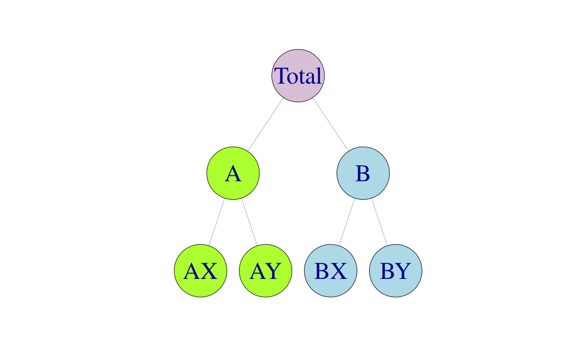
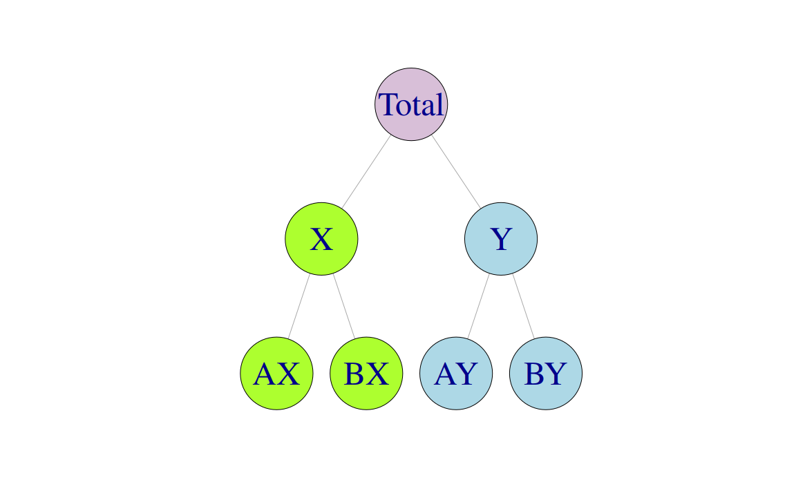
Figure 10.4: Alternative representations of a two level grouped structure.
This example shows that there are alternative aggregation paths for grouped structures. For any time \(t\), as with the hierarchical structure, \[\begin{equation*} y_{t}=\y{AX}{t}+\y{AY}{t}+\y{BX}{t}+\y{BY}{t}. \end{equation*}\] However, for the first level of the grouped structure, \[\begin{equation} \y{A}{t}=\y{AX}{t}+\y{AY}{t}\quad \quad \y{B}{t}=\y{BX}{t}+\y{BY}{t} \tag{10.4} \end{equation}\] but also \[\begin{equation} \y{X}{t}=\y{AX}{t}+\y{BX}{t}\quad \quad \y{Y}{t}=\y{AY}{t}+\y{BY}{t} \tag{10.5}. \end{equation}\]
These equalities can again be represented by the summing matrix \(\bm{S}\) which recall is of dimension \(n\times m\). The total number of series is \(n=9\) with \(m=4\) series at the bottom-level. For the grouped structure in Figure 10.4 we write \[ \begin{bmatrix} y_{t} \\ \y{A}{t} \\ \y{B}{t} \\ \y{X}{t} \\ \y{Y}{t} \\ \y{AX}{t} \\ \y{AY}{t} \\ \y{BX}{t} \\ \y{BY}{t} \end{bmatrix} = \begin{bmatrix} 1 & 1 & 1 & 1 \\ 1 & 1 & 0 & 0 \\ 0 & 0 & 1 & 1 \\ 1 & 0 & 1 & 0 \\ 0 & 1 & 0 & 1 \\ 1 & 0 & 0 & 0 \\ 0 & 1 & 0 & 0 \\ 0 & 0 & 1 & 0 \\ 0 & 0 & 0 & 1 \end{bmatrix} \begin{bmatrix} \y{AX}{t} \\ \y{AY}{t} \\ \y{BX}{t} \\ \y{BY}{t} \end{bmatrix} \] where now the second and third rows of \(\bm{S}\) represent (10.4) and the fourth and fifth rows represent (10.5).
Grouped time series can be thought of as hierarchical time series that do not impose a unique hierarchical structure in the sense that the order by which the series can be grouped is not unique.
Example: Australian prison population
The left plot in the top row of Figure 10.5 shows the total number of prisoners in Australia over the period 2005 Q1 to 2016 Q4. This represents the top-level series in the grouping structure. The rest of the plots show the prison population grouped by (i) state18 (ii) legal status, whether prisoners have already been sentenced or are in remand waiting for a sentence, and (iii) gender.
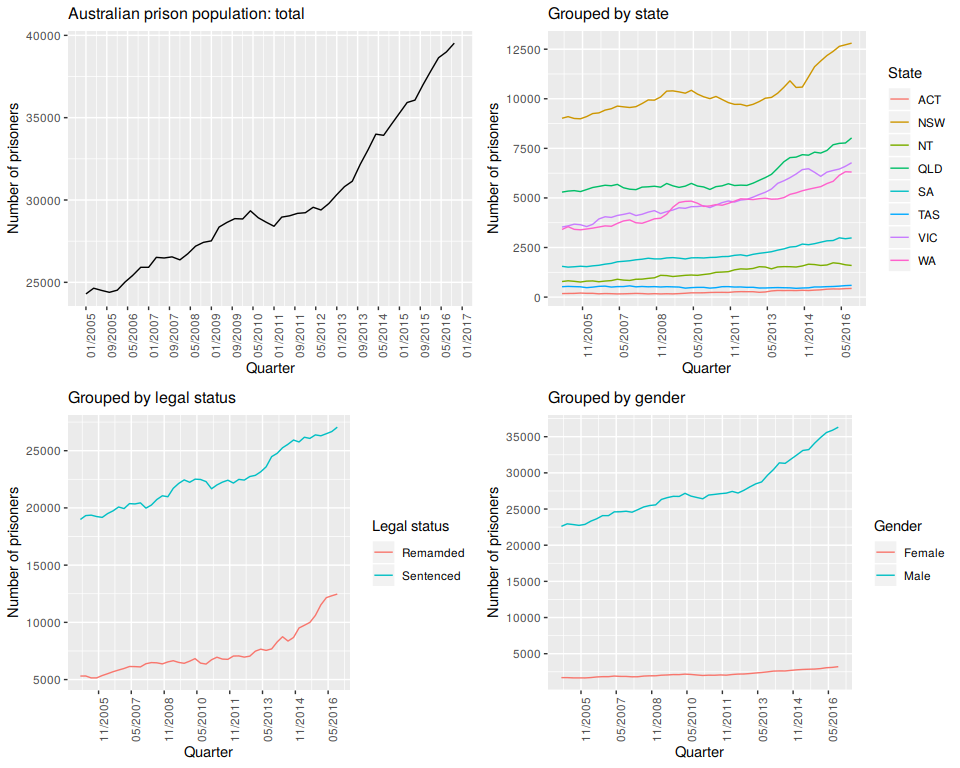
Figure 10.5: Total Australian adult prison population and Australian prison population grouped by state, by legal status and by gender.
To create a grouped time series we use the gts function as shown below. Similarly to the hts function the gts function requires as inputs the bottom-level time series and information about the grouping structure. prison is a time series matrix containing the bottom-level times series. Similarly to the hts function the information about the grouping structure can be passed in using the characters input. An alternative is to be more explicit about the labelling of the series and use the groups input. The code below shows examples for both these.
TODO: talk about interactions here - but possibly need to wait for update of the hts
prison <- read.csv("Ch10Data/prison.csv", strip.white = TRUE, check.names=FALSE)
prison <- ts(prison, start=c(2005,1), end=c(2016,4), frequency=4)
# Need to make data into prison time series matrix to add to fpp2

# Using the `characters` input
prison.gts <- gts(prison, characters = c(1,1,1))
#> Argument gnames is missing and the default labels are used.

# Using the `groups` input # 8 states, 2 legal, 2 gender
s <- rep(c("NSW", "VIC", "QLD", "SA", "WA", "NT", "ACT", "TAS"), 32/8)
l <- rep(rep(c("Rem","Sen"),each=8),2) # Sentenced is number 2 here
g <- rep(c("M","F"),each=32/2)
s_l <- as.character(interaction(s,l,sep=""))
s_g <- as.character(interaction(s,g,sep=""))
g_l <- as.character(interaction(g,l,sep=""))
gc <-rbind(s,l,g,s_l, s_g, g_l)
prison.gts <- gts(prison,groups=gc)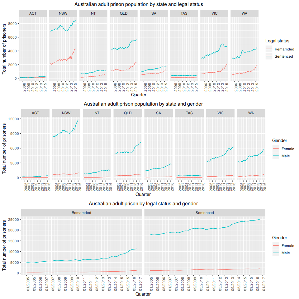
Figure 10.6: Australian adult prison population grouped by pairs of attributes.
Figure 10.7 shows the Australian adult population grouped by all three attributes: state, legal status and gender. These form the bottom-level series of the grouped structure for the Australian prison population.
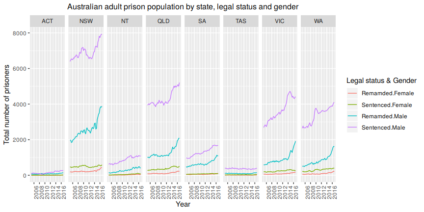
Figure 10.7: Bottom-level time series for the Australian adult prison population, grouped by state, legal status and gender.
Australia comprises eight geographical areas six states and two territories: Australian Capital Territory, New South Wales, Northern Terrirory, Queensland, South Australia, Tasmania, Victoria, Western Australia. In this example we consider all eight.↩