12.10 Multi-step forecasts on training data

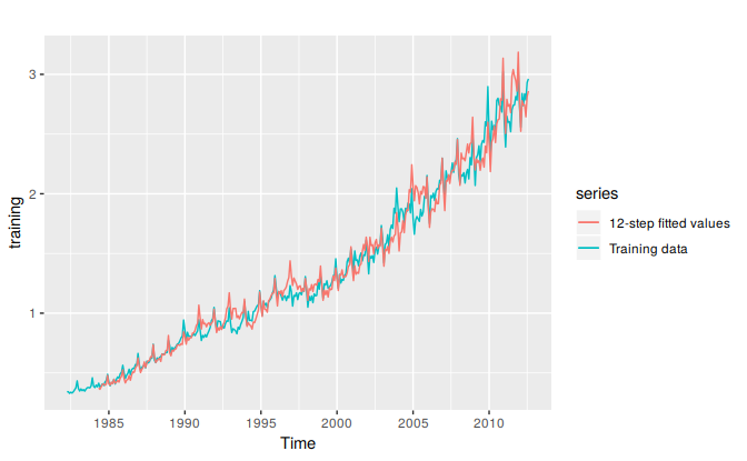
Just as it is useful to obtain one-step forecasts on the test set, it is sometimes useful to compute multi-step forecasts on the training set. We normally define fitted values to be one-step forecasts on the training set (see Section 3.3), but a similar idea can be used for multi-step forecasts. The fitted() function has an h argument to allow for \(h\)-step “fitted values” on the training set.

Here is a plot of 12-step (one year) forecasts on the training set used for the model of Australian eating-out expenditure in the previous section. Because the model involves both seasonal (lag 12) and first (lag 1) differencing, it is not possible to compute these forecasts for the first 25 observations.

autoplot(training, series="Training data") +
  forecast::autolayer(fitted(cafe.train, h=12), series="12-step fitted values")