8.10 ARIMA vs ETS
It is a commonly held myth that ARIMA models are more general than exponential smoothing. While linear exponential smoothing models are all special cases of ARIMA models, the non-linear exponential smoothing models have no equivalent ARIMA counterparts. On the other hand, there are also many ARIMA models that have no exponential smoothing counterparts. In particular, all ETS models are non-stationary, while some ARIMA models are stationary.
The ETS models with seasonality or non-damped trend or both have two unit roots (i.e., they need two levels of differencing to make them stationary). All other ETS models have one unit root (they need one level of differencing to make them stationary).
The following table gives the equivalence relationships for the two classes of models.
| ETS model | ARIMA model | Parameters |
|---|---|---|
| ETS(A,N,N) | ARIMA(0,1,1) | \(\theta_1 = \alpha-1\) |
| ETS(A,A,N) | ARIMA(0,2,2) | \(\theta_1 = \alpha+\beta-2\) |
| \(\theta_2 = 1-\alpha\) | ||
| ETS(A,A,N) | ARIMA(1,1,2) | \(\phi_1=\phi\) |
| \(\theta_1 = \alpha+\phi\beta-1-\phi\) | ||
| \(\theta_2 = (1-\alpha)\phi\) | ||
| ETS(A,N,A) | ARIMA(0,0,\(m\))(0,1,0)\(_m\) | |
| ETS(A,A,A) | ARIMA(0,1,\(m+1\))(0,1,0)\(_m\) | |
| ETS(A,A,A) | ARIMA(1,0,\(m+1\))(0,1,0)\(_m\) |
For the seasonal models, the ARIMA parameters have a large number of restrictions.
The AICc is useful for selecting between models in the same class. For example, we can use it to select an ARIMA model between candidate ARIMA models16 or an ETS model between candidate ETS models. However, it cannot be used to compare between ETS and ARIMA models because they are in different model classes, and the likelihood is computed in different ways. The examples below demonstrate selecting between these classes of models.
Example: Comparing auto.arima() and ets() on non-seasonal data
We can use time series cross-validation to compare an ARIMA model and an ETS model. The code below provides functions that return forecast objects from auto.arima() and ets() respectively.
fets <- function(x, h) {
  forecast(ets(x), h = h)
}
farima <- function(x, h) {
  forecast(auto.arima(x), h=h)
}
The returned objects can then be passed into tsCV. Let’s consider ARIMA models and ETS models for the air data as introduced in Section 7.2 where, air <- window(ausair, start=1990).
# Compute CV errors for ETS as e1
e1 <- tsCV(air, fets, h=1)
# Compute CV errors for ARIMA as e2
e2 <- tsCV(air, farima, h=1)
# Find MSE of each model class
mean(e1^2, na.rm=TRUE)
#> [1] 7.86
mean(e2^2, na.rm=TRUE)
#> [1] 9.62
In this case the ets model has a lower tsCV statistic based on MSEs. Below we generate and plot forecasts for the next 5 years generated from an ets model.
air %>% ets() %>% forecast() %>% autoplot()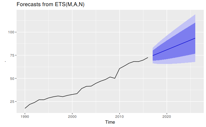
Example: Comparing auto.arima() and ets() on seasonal data
In this case we want to compare seasonal ARIMA and ETS models applied to the quarterly cement production data qcement. Because the series is very long, we can afford to use a training and a test set rather than time series cross-validation. The advantage is that this is much faster. We create a training set from the beginning of 1988 to the end of 2007 and select an ARIMA and an ETS model using the auto.arima and ets functions.
# Consider the qcement data beginning in 1988
cement <- window(qcement, start=1988)
# Use 20 years of the data as the training set
train <- window(cement, end=c(2007,4))
The output below shows the ARIMA model selected and estimated by auto.arima. The ARIMA model does well in capturing all the dynamics in the data as the residuals seem to be white noise.
# Fit an ARIMA model to the training data
(fit.arima <- auto.arima(train))
#> Series: train
#> ARIMA(1,0,1)(2,1,1)[4] with drift
#>
#> Coefficients:
#>         ar1     ma1   sar1    sar2    sma1  drift
#>       0.889  -0.237  0.081  -0.235  -0.898  0.010
#> s.e.  0.084   0.133  0.157   0.139   0.178  0.003
#>
#> sigma^2 estimated as 0.0115:  log likelihood=61.5
#> AIC=-109   AICc=-107   BIC=-92.6
checkresiduals(fit.arima)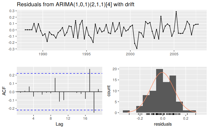
#>
#>  Ljung-Box test
#>
#> data:  Residuals from ARIMA(1,0,1)(2,1,1)[4] with drift
#> Q* = 3, df = 3, p-value = 0.3
#>
#> Model df: 6.   Total lags used: 9
The output below also shows the ETS model selected and estimated by ets. This models also does well in capturing all the dynamics in the data as the residuals also seem to be white noise.
# Fit an ETS model to the training data
(fit.ets <- ets(train))
#> ETS(M,N,M)
#>
#> Call:
#>  ets(y = train)
#>
#>   Smoothing parameters:
#>     alpha = 0.7341
#>     gamma = 1e-04
#>
#>   Initial states:
#>     l = 1.6439
#>     s = 1.03 1.04 1.01 0.915
#>
#>   sigma:  0.0581
#>
#>    AIC   AICc    BIC
#> -2.197 -0.641 14.477
checkresiduals(fit.ets)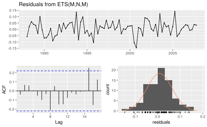
#>
#>  Ljung-Box test
#>
#> data:  Residuals from ETS(M,N,M)
#> Q* = 6, df = 3, p-value = 0.1
#>
#> Model df: 6.   Total lags used: 9
The output below evaluates the forecasting performance of the two competing models over the test set. In this case the ETS model seems to be the slighlty more accuarate model based on the test set RMSE, MAPE and MASE.
# Generate forecasts and compare accuracy over the test set
fit.arima %>% forecast(h = 4*(2013-2007)+1) %>% accuracy(qcement)
#>                    ME RMSE    MAE   MPE MAPE  MASE    ACF1 Theil's U
#> Training set -0.00621  0.1 0.0799 -0.67 4.37 0.546 -0.0113        NA
#> Test set     -0.15884  0.2 0.1688 -7.33 7.72 1.153  0.2917     0.728
fit.ets %>% forecast(h = 4*(2013-2007)+1) %>% accuracy(qcement)
#>                   ME  RMSE    MAE    MPE MAPE  MASE    ACF1 Theil's U
#> Training set  0.0141 0.102 0.0796  0.494 4.37 0.544 -0.0335        NA
#> Test set     -0.1350 0.184 0.1540 -6.251 6.99 1.052  0.5344     0.681
Below we generate and plot forecasts from an ets model for the next 3 years.
# Generate forecasts from an ETS model
cement %>% ets() %>% forecast(h=12) %>% autoplot()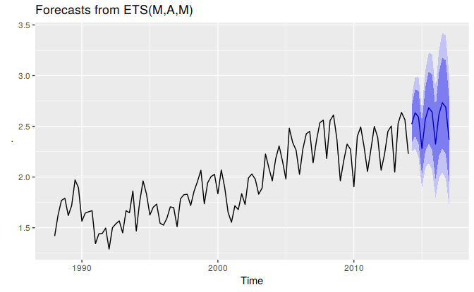
As already pointed out, comparing information criteria is only valid for ARIMA models of the same orders of differencing.↩