6.7 Forecasting with decomposition

While decomposition is primarily useful for studying time series data, and exploring the historical changes over time, it can also be used in forecasting.

Assuming an additive decomposition, the decomposed time series can be written as \[ y_t = \hat{S}_t + \hat{A}_t, \] where \(\hat{A}_t = \hat{T}_t+\hat{R}_{t}\) is the seasonally adjusted component. Or, if a multiplicative decomposition has been used, we can write \[ y_t = \hat{S}_t\hat{A}_t, \] where \(\hat{A}_t = \hat{T}_t\hat{R}_{t}\).

To forecast a decomposed time series, we forecast the seasonal component, \(\hat{S}_t\), and the seasonally adjusted component \(\hat{A}_t\), separately. It is usually assumed that the seasonal component is unchanging, or changing extremely slowly, so it is forecast by simply taking the last year of the estimated component. In other words, a seasonal naïve method is used for the seasonal component.

To forecast the seasonally adjusted component, any non-seasonal forecasting method may be used. For example, a random walk with drift model, or Holt’s method (discussed in the next chapter), or a non-seasonal ARIMA model (discussed in Chapter 8), may be used.

Example: Electrical equipment manufacturing

fit <- stl(elecequip, t.window=13, s.window="periodic", robust=TRUE)

fit %>% seasadj() %>% naive() %>% autoplot() + ylab("New orders index") +
  ggtitle("Naive forecasts of seasonally adjusted data")

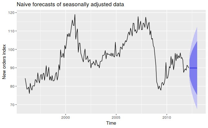
Figure 6.14: Naïve forecasts of the seasonally adjusted data obtained from an STL decomposition of the electrical equipment orders data.

Figure 6.14 shows naïve forecasts of the seasonally adjusted electrical equipment orders data. These are then “reseasonalized” by adding in the seasonal naïve forecasts of the seasonal component.

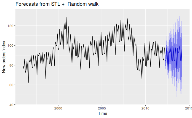
This is made easy with the forecast function applied to the stl object. You need to specify the method being used on the seasonally adjusted data, and the function will do the re-seasonalizing for you. The resulting forecasts of the original data are shown in Figure 6.15.

fit %>% forecast(method="naive") %>% autoplot() + ylab("New orders index")

Figure 6.15: Forecasts of the electrical equipment orders data based on a naïve forecast of the seasonally adjusted data and a seasonal naïve forecast of the seasonal component, after an STL decomposition of the data.

The prediction intervals shown in this graph are constructed in the same way as the point forecasts. That is, the upper and lower limits of the prediction intervals on the seasonally adjusted data are “reseasonalized” by adding in the forecasts of the seasonal component. In this calculation, the uncertainty in the forecasts of the seasonal component has been ignored. The rationale for this choice is that the uncertainty in the seasonal component is much smaller than that for the seasonally adjusted data, and so it is a reasonable approximation to ignore it.

A short-cut approach is to use the stlf function. The following code will decompose the time series using STL, forecast the seasonally adjusted series, and return reseasonalize the forecasts.

fcast <- stlf(eeadj, method='naive')

The stlf function uses default values for s.window and t.window.

As well as the naïve method, several other possible forecasting methods are available with stlf, as described in the corresponding help file. If method is not specified, it will use the ETS approach (discussed in the next chapter) applied to the seasonally adjusted series. This usually produces quite good forecasts for seasonal time series, and some companies use it routinely for all their operational forecasts.