5.1 The linear model

Simple linear regression

In the simplest case, there is a linear relationship between the forecast variable and a single predictor variable, \[ y_t = \beta_0 + \beta_1 x_t + \varepsilon_t. \] An example of data from such a model is shown in Figure 5.1. The parameters \(\beta_0\) and \(\beta_1\) denote the intercept and the slope of the line respectively. The intercept \(\beta_0\) represents the predicted value of \(y\) when \(x=0\). The slope \(\beta_1\) represents the average predicted change in \(y\) resulting from a one unit increase in \(x\).

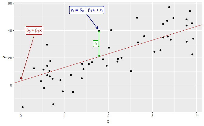
Figure 5.1: An example of data from a linear regression model.

Notice that the observations do not lie on the straight line but are scattered around it. We can think of each observation \(y_t\) consisting of the systematic or explained part of the model, \(\beta_0+\beta_1x_t\), and the random “error”, \(\varepsilon_t\). The “error” term does not imply a mistake, but a deviation from the underlying straight line model. It captures anything that may affect \(y_t\) other than \(x_t\).

Example: US consumption expenditure

Figure 5.2 shows time series of quarterly percentage changes (growth rates) of real personal consumption expenditure (\(y\)) and real personal disposable income (\(x\)) for the US from 1970 Q1 to 2016 Q3.

autoplot(uschange[,c("Consumption","Income")]) +
  ylab("% change") + xlab("Year")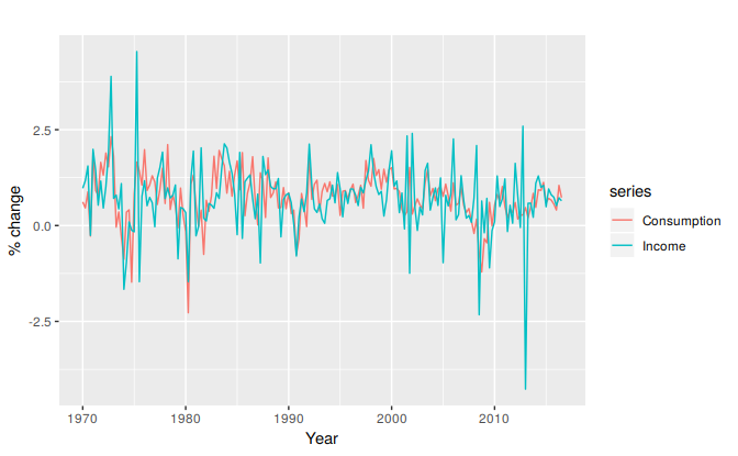

Figure 5.2: Percentage changes in personal consumption expenditure and personal income for the US.

A scatter plot of consumption against income is shown in Figure 5.3 along with the estimated regression line \[ \hat{y}_t=0.55 + 0.28x_t. \] (We put a “hat” above the \(y\) to indicate this is an estimate or prediction.)

uschange %>%
  as.data.frame() %>%
  ggplot(aes(x=Income, y=Consumption)) +
    ylab("Consumption (quarterly % change)") +
    xlab("Income (quarterly % change)") +
    geom_point() +
    geom_smooth(method="lm", se=FALSE)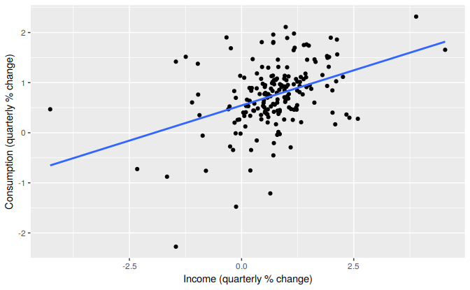

Figure 5.3: Scatterplot of consumption versus income and the fitted regression line.

This equation is estimated in R using the tslm function:

tslm(Consumption ~ Income, data=uschange)
#> 
#> Call:
#> tslm(formula = Consumption ~ Income, data = uschange)
#> 
#> Coefficients:
#> (Intercept)       Income  
#>       0.545        0.281

We will discuss how tslm computes the coefficients in Section 5.2.

The fitted line has a positive slope, reflecting the positive relationship between income and consumption. The slope coefficient shows that a one unit increase in \(x\) (a 1% increase in personal disposable income) results on average in 0.28 units increase in \(y\) (an average 0.28% increase in personal consumption expenditure). Alternatively the estimated equation shows that a value of 1 for \(x\) (the percentage increase in personal disposable income) will result in a forecast value of \(0.55 + 0.28 \times 1 = 0.83\) for \(y\) (the percentage increase in personal consumption expenditure).

The interpretation of the intercept requires that a value of \(x=0\) makes sense. In this case when \(x=0\) (i.e., when there is no change in personal disposable income since the last quarter) the predicted value of \(y\) is 0.55 (i.e., an average increase in personal consumption expenditure of 0.55%). Even when \(x=0\) does not make sense, the intercept is an important part of the model. Without it, the slope coefficient can be distorted unnecessarily. The intercept should always be included unless the requirement is to force the regression line “through the origin”. In what follows we assume that an intercept is always included in the model.

Multiple linear regression

When there are two or more predictor variables, the model is called a “multiple regression model”. The general form of a multiple regression model is \[\begin{equation} y_t = \beta_{0} + \beta_{1} x_{1,t} + \beta_{2} x_{2,t} + \cdots + \beta_{k} x_{k,t} + \varepsilon_t, \tag{5.1} \end{equation}\] where \(y\) is the variable to be forecast and \(x_{1},\dots,x_{k}\) are the \(k\) predictor variables. Each of the predictor variables must be numerical. The coefficients \(\beta_{1},\dots,\beta_{k}\) measure the effect of each predictor after taking account of the effect of all other predictors in the model. Thus, the coefficients measure the marginal effects of the predictor variables.

Example: US consumption expenditure (revisited)

Figure 5.4 shows additional predictors that may be useful for forecasting US consumption expenditure. These are quarterly percentage changes in industrial production and personal savings, and quarterly changes in the unemployment rate (as this is already a percentage). Building a multiple linear regression model can potentially generate more accurate forecasts as we expect consumption expenditure to not only depend on personal income but on other predictors as well.

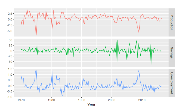
Figure 5.4: Quarterly percentage changes in industrial production and personal savings and quarterly changes in the unemployment rate for the US over the period 1960Q1-2016Q3.

The first column of Figure 5.5 below shows the relationships between consumption and each of the predictors. The scatterplots show positive relationships with income and industrial production, and negative relationships with savings and unemployment. The strength of these relationships are shown by the correlation coefficients across the first row. The remaining scatterplots and correlation coefficients show the relationships between the predictors.

uschange %>%
  as.data.frame() %>%
  GGally::ggpairs()
#> Registered S3 method overwritten by 'GGally':
#>   method from   
#>   +.gg   ggplot2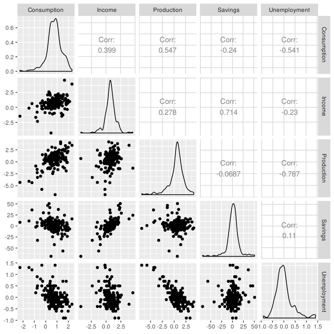

Figure 5.5: A scatterplot matrix of US consumption expenditure and the four predictors.

Assumptions

When we use a linear regression model, we are implicitly making some assumptions about the variables in Equation (5.1).

First, we assume that the model is a reasonable approximation to reality; that is, that the relationship between the forecast variable and the predictor variables satisfies this linear equation.

Second, we make the following assumptions about the errors \((\varepsilon_{1},\dots,\varepsilon_{T})\):

• they have mean zero; otherwise the forecasts will be systematically biased.
• they are not autocorrelated; otherwise the forecasts will be inefficient as there is more information to be exploited in the data.
• they are unrelated to the predictor variables; otherwise there would be more information that should be included in the systematic part of the model.

It is also useful to have the errors that are normally distributed with constant variance \(\sigma^2\) in order to easily produce prediction intervals.

Another important assumption in the linear regression model is that each predictor \(x\) is not a random variable. If we were performing a controlled experiment in a laboratory, we could control the values of each \(x\) (so they would not be random) and observe the resulting values of \(y\). With observational data (including most data in business and economics) it is not possible to control the value of \(x\), and hence we make this an assumption.