2.4 Seasonal plots

A seasonal plot is similar to a time plot except that the data are plotted against the individual “seasons” in which the data were observed. An example is given below showing the antidiabetic drug sales.

ggseasonplot(a10, year.labels=TRUE, year.labels.left=TRUE) +
  ylab("$ million") + ggtitle("Seasonal plot: antidiabetic drug sales")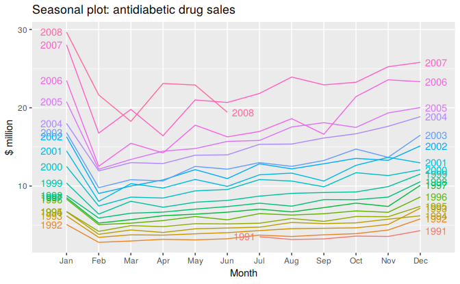

Figure 2.4: Seasonal plot of monthly antidiabetic drug sales in Australia.

These are exactly the same data as were shown earlier, but now the data from each season are overlapped. A seasonal plot allows the underlying seasonal pattern to be seen more clearly, and is especially useful in identifying years in which the pattern changes.

In this case, it is clear that there is a large jump in sales in January each year. Actually, these are probably sales in late December as customers stockpile before the end of the calendar year, but the sales are not registered with the government until a week or two later. The graph also shows that there was an unusually small number of sales in March 2008 (most other years show an increase between February and March). The small number of sales in June 2008 is probably due to incomplete counting of sales at the time the data were collected.

A useful variation on the seasonal plot uses polar coordinates. Setting polar=TRUE makes the time series axis circular rather than horizontal, as shown below.

ggseasonplot(a10, polar=TRUE) +
  ylab("$ million") + ggtitle("Polar seasonal plot: antidiabetic drug sales")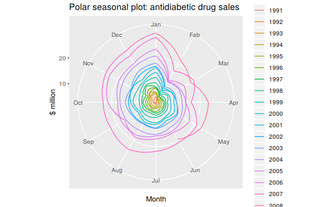

Figure 2.5: Polar seasonal plot of monthly antidiabetic drug sales in Australia.