5.3 Some useful predictors
There are several very useful predictors that occur frequently when using regression for time series data.
Trend
It is very common for time series data to be trending. A linear trend can be modelled by simply using \(x_{1,t}=t\) as a predictor,
\[
y_{t}= \beta_0+\beta_1t+\varepsilon_t,
\]
where \(t=1,\dots,T\). A trend variable can be specified in the tslm function using the trend predictor. In Section 5.8 we discuss how we can also model a nonlinear trends.
Dummy variables
So far, we have assumed that each predictor takes numerical values. But what about when a predictor is a categorical variable taking only two values (e.g., “yes” and “no”). Such a variable might arise, for example, when forecasting daily sales and you want to take account of whether the day is a public holiday or not. So the predictor takes value “yes” on a public holiday, and “no” otherwise.
This situation can still be handled within the framework of multiple regression models by creating a “dummy variable” taking value 1 corresponding to “yes” and 0 corresponding to “no”. A dummy variable is also known as an “indicator variable”.
A dummy variable can also be used to account for an outlier in the data. Rather than omit the outlier, a dummy variable removes its effect. In this case, the dummy variable takes value 1 for that observation and 0 everywhere else. An example is the case where a special event has occurred. For example when forecasting tourist arrivals to Brazil, we will need to account for the effect of the Rio de Janeiro summer Olympics in 2016.
If there are more than two categories, then the variable can be coded using several dummy variables (one fewer than the total number of categories). tslm will automatically handle this case if you specify a factor variable as a predictor. There is usually no need to manually create the corresponding dummy variables.
Seasonal dummy variables
For example, suppose we are forecasting daily electricity demand and we want to account for the day of the week as a predictor. Then the following dummy variables can be created.
| \(d_{1,t}\) | \(d_{2,t}\) | \(d_{3,t}\) | \(d_{4,t}\) | \(d_{5,t}\) | \(d_{6,t}\) | |
|---|---|---|---|---|---|---|
| Monday | 1 | 0 | 0 | 0 | 0 | 0 |
| Tuesday | 0 | 1 | 0 | 0 | 0 | 0 |
| Wednesday | 0 | 0 | 1 | 0 | 0 | 0 |
| Thursday | 0 | 0 | 0 | 1 | 0 | 0 |
| Friday | 0 | 0 | 0 | 0 | 1 | 0 |
| Saturday | 0 | 0 | 0 | 0 | 0 | 1 |
| Sunday | 0 | 0 | 0 | 0 | 0 | 0 |
| Monday | 1 | 0 | 0 | 0 | 0 | 0 |
| Tuesday | 0 | 1 | 0 | 0 | 0 | 0 |
| Wednesday | 0 | 0 | 1 | 0 | 0 | 0 |
| Thursday | 0 | 0 | 0 | 1 | 0 | 0 |
| Friday | 0 | 0 | 0 | 0 | 1 | 0 |
| ⋮ | ⋮ | ⋮ | ⋮ | ⋮ | ⋮ | ⋮ |
Notice that only six dummy variables are needed to code seven categories. That is because the seventh category (in this case Sunday) is specified when all dummy variables are all set to zero and is captured by the intercept.
Many beginners will try to add a seventh dummy variable for the seventh category. This is known as the “dummy variable trap” because it will cause the regression to fail. There will be one too many parameters to estimate when an intercept is also included. The general rule is to use one fewer dummy variables than categories. So for quarterly data, use three dummy variables; for monthly data, use 11 dummy variables; and for daily data, use six dummy variables, and so on.
The interpretation of each of the coefficients associated with the dummy variables is that it is a measure of the effect of that category relative to the omitted category. In the above example, the coefficient of \(d_{1,t}\) associated with Monday will measure the effect of Monday compared to Sunday on the forecast variable. An example of interpreting estimated dummy variable coefficients capturing the quarterly seasonality of Australian beer production follows.
The tslm function will automatically handle this situation if you specify the predictor season.
Example: Australian quarterly beer production
Recall the Australian quarterly beer production data shown again in Figure 5.8 below.
beer2 <- window(ausbeer, start=1992)
autoplot(beer2) + xlab("Year") + ylab("Megalitres")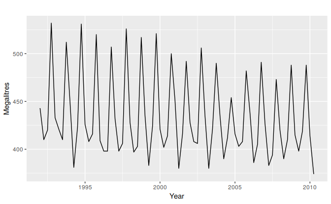
Figure 5.8: Australian quarterly beer production.
We want to forecast the value of future beer production. We can model this data using a regression model with a linear trend and quarterly dummy variables, \[ y_{t} = \beta_{0} + \beta_{1} t + \beta_{2}d_{2,t} + \beta_3 d_{3,t} + \beta_4 d_{4,t} + \varepsilon_{t}, \] where \(d_{i,t} = 1\) if \(t\) is in quarter \(i\) and 0 otherwise. The first quarter variable has been omitted, so the coefficients associated with the other quarters are measures of the difference between those quarters and the first quarter.
fit.beer <- tslm(beer2 ~ trend + season)
summary(fit.beer)
#>
#> Call:
#> tslm(formula = beer2 ~ trend + season)
#>
#> Residuals:
#>    Min     1Q Median     3Q    Max
#> -42.90  -7.60  -0.46   7.99  21.79
#>
#> Coefficients:
#>             Estimate Std. Error t value Pr(>|t|)
#> (Intercept) 441.8004     3.7335  118.33  < 2e-16 ***
#> trend        -0.3403     0.0666   -5.11  2.7e-06 ***
#> season2     -34.6597     3.9683   -8.73  9.1e-13 ***
#> season3     -17.8216     4.0225   -4.43  3.4e-05 ***
#> season4      72.7964     4.0230   18.09  < 2e-16 ***
#> ---
#> Signif. codes:  0 '***' 0.001 '**' 0.01 '*' 0.05 '.' 0.1 ' ' 1
#>
#> Residual standard error: 12.2 on 69 degrees of freedom
#> Multiple R-squared:  0.924,  Adjusted R-squared:  0.92
#> F-statistic:  211 on 4 and 69 DF,  p-value: <2e-16
Note that trend and season are not objects in the R workspace; they are created automatically by tslm when specified in this way.
There is a downward trend of -0.34 megalitres per quarter. On average, the second quarter has production of 34.7 megalitres lower than the first quarter, the third quarter has production of 17.8 megalitres lower than the first quarter, and the fourth quarter has production of 72.8 megalitres higher than the first quarter.
autoplot(beer2, series="Data") +
  forecast::autolayer(fitted(fit.beer), series="Fitted") +
  xlab("Year") + ylab("Megalitres") +
  ggtitle("Quarterly Beer Production")
Figure 5.9: Time plot of beer production and predicted beer production.
cbind(Data=beer2, Fitted=fitted(fit.beer)) %>%
  as.data.frame() %>%
  ggplot(aes(x=Data, y=Fitted, colour=as.factor(cycle(beer2)))) +
    geom_point() +
    ylab("Fitted") + xlab("Actual values") +
    ggtitle("Quarterly beer production") +
    scale_colour_brewer(palette="Dark2", name="Quarter") +
    geom_abline(intercept=0, slope=1)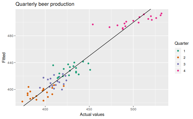
Figure 5.10: Actual beer production plotted against predicted beer production.
Fourier series
An alternative to using seasonal dummy variables, especially for long seasonal periods, is to use Fourier terms. Jean-Baptiste Fourier was a French mathematician, born in the 1700s, who showed that a series of sine and cosine terms of the right frequencies can approximate any periodic function. We can use them for seasonal patterns.
If \(m\) is the seasonal period, then the first few Fourier terms are given by \[ x_{1,t} = \sin\left(\textstyle\frac{2\pi t}{m}\right), x_{2,t} = \cos\left(\textstyle\frac{2\pi t}{m}\right), x_{3,t} = \sin\left(\textstyle\frac{4\pi t}{m}\right), x_{4,t} = \cos\left(\textstyle\frac{4\pi t}{m}\right), x_{5,t} = \sin\left(\textstyle\frac{6\pi t}{m}\right), x_{6,t} = \cos\left(\textstyle\frac{6\pi t}{m}\right), \] and so on. If we have monthly seasonality, and we use the first 11 of these predictor variables, then we will get exactly the same forecasts as using 11 dummy variables.
The advantage of using Fourier terms is that we can often use fewer predictor variables than we need to with dummy variables, especially when \(m\) is large. This makes them useful for weekly data, for example, where \(m\approx 52\). For short seasonal periods such as with quarterly data, there is little advantage in using Fourier series over seasonal dummy variables.
In R, these Fourier terms are produced using the fourier function. For example, the Australian beer data can be modelled like this.
fourier.beer <- tslm(beer2 ~ trend + fourier(beer2, K=2))
summary(fourier.beer)
#>
#> Call:
#> tslm(formula = beer2 ~ trend + fourier(beer2, K = 2))
#>
#> Residuals:
#>    Min     1Q Median     3Q    Max
#> -42.90  -7.60  -0.46   7.99  21.79
#>
#> Coefficients:
#>                           Estimate Std. Error t value Pr(>|t|)
#> (Intercept)               446.8792     2.8732  155.53  < 2e-16 ***
#> trend                      -0.3403     0.0666   -5.11  2.7e-06 ***
#> fourier(beer2, K = 2)S1-4   8.9108     2.0112    4.43  3.4e-05 ***
#> fourier(beer2, K = 2)C1-4  53.7281     2.0112   26.71  < 2e-16 ***
#> fourier(beer2, K = 2)C2-4  13.9896     1.4226    9.83  9.3e-15 ***
#> ---
#> Signif. codes:  0 '***' 0.001 '**' 0.01 '*' 0.05 '.' 0.1 ' ' 1
#>
#> Residual standard error: 12.2 on 69 degrees of freedom
#> Multiple R-squared:  0.924,  Adjusted R-squared:  0.92
#> F-statistic:  211 on 4 and 69 DF,  p-value: <2e-16
The first argument to fourier just allows it to identify the seasonal period \(m\) and the length of the predictors to return. The second K argument specifies how many pairs of sin and cos terms to include. The maximum number allowed is \(K=m/2\) where \(m\) is the seasonal period. Because we have used the maximum here, the results are identical to those obtained when using seasonal dummy variables.
If only the first two Fourier terms are used (\(x_{1,t}\) and \(x_{2,t}\)), the seasonal pattern will follow a simple sine wave. A regression model containing Fourier terms is often called a harmonic regression because the successive Fourier terms represent harmonics of the first two Fourier terms.
Intervention variables
It is often necessary to model interventions that may have affected the variable to be forecast. For example, competitor activity, advertising expenditure, industrial action, and so on, can all have an effect.
When the effect lasts only for one period, we use a spike variable. This is a dummy variable taking value one in the period of the intervention and zero elsewhere. A spike variable is equivalent to a dummy variable for handling an outlier.
Other interventions have an immediate and permanent effect. If an intervention causes a level shift (i.e., the value of the series changes suddenly and permanently from the time of intervention), then we use a step variable. A step variable takes value zero before the intervention and one from the time of intervention onward.
Another form of permanent effect is a change of slope. Here the intervention is handled using a piecewise linear trend; a trend that bends at the time of intervention and hence is nonlinear. We will discuss this in Section 5.8.
Trading days
The number of trading days in a month can vary considerably and can have a substantial effect on sales data. To allow for this, the number of trading days in each month can be included as a predictor.
For monthly or quarterly data, the bizdays function will compute the number of trading days in each period.
An alternative that allows for the effects of different days of the week has the following predictors:
Distributed lags
It is often useful to include advertising expenditure as a predictor. However, since the effect of advertising can last beyond the actual campaign, we need to include lagged values of advertising expenditure. So the following predictors may be used. \[\begin{align*} x_{1} &= \text{advertising for previous month;} \\ x_{2} &= \text{advertising for two months previously;} \\ & \vdots \\ x_{m} &= \text{advertising for $m$ months previously.} \end{align*}\]
It is common to require the coefficients to decrease as the lag increases, although this is beyond the scope of this book.
Easter
Easter is different from most holidays because it is not held on the same date each year and the effect can last for several days. In this case, a dummy variable can be used with value one where the holiday falls in the particular time period and zero otherwise.
For example, with monthly data, when Easter falls in March then the dummy variable takes value 1 in March, when it falls in April, the dummy variable takes value 1 in April, and when it starts in March and finishes in April, the dummy variable is split proportionally between months.
The easter function will compute the dummy variable for you.