5.2 Least squares estimation

In practice, of course, we have a collection of observations but we do not know the values of the coefficients \(\beta_0,\beta_1, \dots, \beta_k\). These need to be estimated from the data.

The least squares principle provides a way of choosing the coefficients effectively by minimizing the sum of the squared errors. That is, we choose the values of \(\beta_0, \beta_1, \dots, \beta_k\) that minimize \[ \sum_{t=1}^T \varepsilon_t^2 = \sum_{t=1}^T (y_t - \beta_{0} - \beta_{1} x_{1,t} - \beta_{2} x_{2,t} - \cdots - \beta_{k} x_{k,t})^2. \]

This is called “least squares” estimation because it gives the least value for the sum of squared errors. Finding the best estimates of the coefficients is often called “fitting” the model to the data, or sometimes “learning” or “training” the model. The line shown in Figure 5.3 was obtained in this way.

When we refer to the estimated coefficients, we will use the notation \(\hat\beta_0, \dots, \hat\beta_k\). The equations for these will be given in Section 5.7.

The tslm function fits a linear regression model to time series data. It is very similar to the lm function which is widely used for linear models, but tslm provides additional facilities for handling time series.

Example: US consumption expenditure (revisited)

A multiple linear regression model for US consumption is \[ y_t=\beta_0 + \beta_1 x_{1,t}+ \beta_2 x_{2,t}+ \beta_3 x_{3,t}+ \beta_4 x_{4,t}+\varepsilon_t, \] where \(y\) is the percentage change in real personal consumption expenditure, \(x_1\) is the percentage change in real personal disposable income, \(x_2\) is the percentage change in industrial production, \(x_3\) is the percentage change in personal savings and \(x_4\) is the change in the unemployment rate.

The following output provides information about the fitted model. The first column of Coefficients gives an estimate of each \(\beta\) coefficient and the second column gives its standard error (i.e., the standard deviation which would be obtained from repeatedly estimating the \(\beta\) coefficients on similar data sets). The standard error gives a measure of the uncertainty in the estimated \(\beta\) coefficient.

fit.consMR <- tslm(Consumption ~ Income + Production + Unemployment + Savings,
  data=uschange)
summary(fit.consMR)
#> 
#> Call:
#> tslm(formula = Consumption ~ Income + Production + Unemployment + 
#>     Savings, data = uschange)
#> 
#> Residuals:
#>     Min      1Q  Median      3Q     Max 
#> -0.8830 -0.1764 -0.0368  0.1525  1.2055 
#> 
#> Coefficients:
#>              Estimate Std. Error t value Pr(>|t|)    
#> (Intercept)   0.26729    0.03721    7.18  1.7e-11 ***
#> Income        0.71448    0.04219   16.93  < 2e-16 ***
#> Production    0.04589    0.02588    1.77    0.078 .  
#> Unemployment -0.20477    0.10550   -1.94    0.054 .  
#> Savings      -0.04527    0.00278  -16.29  < 2e-16 ***
#> ---
#> Signif. codes:  0 '***' 0.001 '**' 0.01 '*' 0.05 '.' 0.1 ' ' 1
#> 
#> Residual standard error: 0.329 on 182 degrees of freedom
#> Multiple R-squared:  0.754,  Adjusted R-squared:  0.749 
#> F-statistic:  139 on 4 and 182 DF,  p-value: <2e-16

For forecasting purposes, the final two columns are of limited interest. The “t value” is the ratio of an estimated \(\beta\) coefficient to its standard error and the last column gives the p-value: the probability of the estimated \(\beta\) coefficient being as large as it is if there was no real relationship between the consumption and the corresponding predictor. This is useful when studying the effect of each predictor, but is not particularly useful when forecasting.

Fitted values

Predictions of \(y\) can be obtained by using the estimated coefficients in the regression equation and setting the error term to zero. In general we write, \[\begin{equation} \hat{y}_t = \hat\beta_{0} + \hat\beta_{1} x_{1,t} + \hat\beta_{2} x_{2,t} + \cdots + \hat\beta_{k} x_{k,t}. \tag{5.2} \end{equation}\] Plugging in the values of \(x_{1,t},\ldots,x_{k,t}\) for \(t=1,\ldots,T\) returns predictions of \(y\) within the training-sample, referred to as fitted values. Note that these are predictions of the data used to estimate the model not genuine forecasts of future values of \(y\).

The following plots show the actual values compared to the fitted values for the percentage change in the US consumption expenditure series. The time plot in Figure 5.6 shows that the fitted values follow the actual data fairly closely. This is verified by the strong positive relationship shown by the scatterplot in Figure 5.7.

autoplot(uschange[,'Consumption'], series="Data") +
  forecast::autolayer(fitted(fit.consMR), series="Fitted") +
  xlab("Year") + ylab("") +
  ggtitle("Percentage change in US consumption expenditure") +
  guides(colour=guide_legend(title=" "))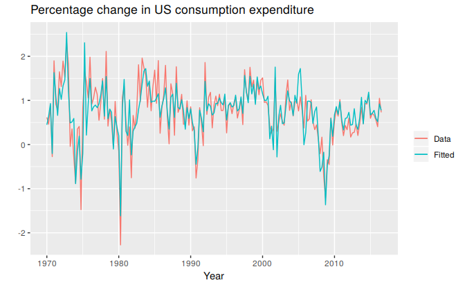

Figure 5.6: Time plot of US consumption expenditure and predicted expenditure.

cbind(Data=uschange[,"Consumption"], Fitted=fitted(fit.consMR)) %>%
  as.data.frame() %>%
  ggplot(aes(x=Data, y=Fitted)) +
    geom_point() +
    xlab("Fitted (predicted values)") +
    ylab("Data (actual values)") +
    ggtitle("Percentage change in US consumption expenditure") +
    geom_abline(intercept=0, slope=1)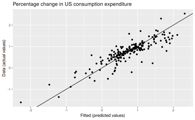

Figure 5.7: Actual US consumption expenditure plotted against predicted US consumption expenditure.