8.3 Autoregressive models

In a multiple regression model, we forecast the variable of interest using a linear combination of predictors. In an autoregression model, we forecast the variable of interest using a linear combination of past values of the variable. The term autoregression indicates that it is a regression of the variable against itself.

Thus, an autoregressive model of order $p$ can be written as \[ y_{t} = c + \phi_{1}y_{t-1} + \phi_{2}y_{t-2} + \dots + \phi_{p}y_{t-p} + e_{t}, \] where $e_t$ is white noise. This is like a multiple regression but with lagged values of $y_t$ as predictors. We refer to this as an AR($p$) model.

Autoregressive models are remarkably flexible at handling a wide range of different time series patterns. The two series in Figure 8.5 show series from an AR(1) model and an AR(2) model. Changing the parameters $\phi_1,\dots,\phi_p$ results in different time series patterns. The variance of the error term $e_t$ will only change the scale of the series, not the patterns.

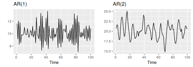
$Two examples of data from autoregressive models with different parameters. Left: AR(1) with $y_t = 18 -0.8y_{t-1} + e_t$. Right: AR(2) with $y_t = 8 + 1.3y_{t-1}-0.7y_{t-2}+e_t$. In both cases, $e_t$ is normally distributed white noise with mean zero and variance one.$

Figure 8.5: Two examples of data from autoregressive models with different parameters. Left: AR(1) with $y_t = 18 -0.8y_{t-1} + e_t$. Right: AR(2) with $y_t = 8 + 1.3y_{t-1}-0.7y_{t-2}+e_t$. In both cases, $e_t$ is normally distributed white noise with mean zero and variance one.

For an AR(1) model:

when $\phi_1=0$, $y_t$ is equivalent to white noise;
when $\phi_1=1$ and $c=0$, $y_t$ is equivalent to a random walk;
when $\phi_1=1$ and $c\ne0$, $y_t$ is equivalent to a random walk with drift;
when $\phi_1<0$, $y_t$ tends to oscillate between positive and negative values;

We normally restrict autoregressive models to stationary data, in which case some constraints on the values of the parameters are required.

For an AR(1) model: $-1 < \phi_1 < 1$.
For an AR(2) model: $-1 < \phi_2 < 1$, $\phi_1+\phi_2 < 1$,

When $p\ge3$, the restrictions are much more complicated. R takes care of these restrictions when estimating a model.