3.1 Some simple forecasting methods

Some forecasting methods are very simple and surprisingly effective. Here are four methods that we will use as benchmarks for other forecasting methods.

Average method

Here, the forecasts of all future values are equal to the mean of the historical data. If we let the historical data be denoted by \(y_{1},\dots,y_{T}\), then we can write the forecasts as \[ \hat{y}_{T+h|T} = \bar{y} = (y_{1}+\dots+y_{T})/T. \] The notation \(\hat{y}_{T+h|T}\) is a short-hand for the estimate of \(y_{T+h}\) based on the data \(y_1,\dots,y_T\).

meanf(y, h)
# y contains the time series
# h is the forecast horizon

###Naïve method {-}

Naïve forecasts are where all forecasts are simply set to be the value of the last observation. That is, \[ \hat{y}_{T+h|T} = y_{T}. \]

This method works remarkably well for many economic and financial time series.

naive(y, h)
rwf(y, h) # Alternative

Seasonal naïve method

A similar method is useful for highly seasonal data. In this case, we set each forecast to be equal to the last observed value from the same season of the year (e.g., the same month of the previous year). Formally, the forecast for time \(T+h\) is written as \[ \hat{y}_{T+h|T} = y_{T+h-km}, \]

where \(m=\) the seasonal period, \(k=\lfloor (h-1)/m\rfloor+1\), and \(\lfloor u \rfloor\) denotes the integer part of \(u\). That looks more complicated than it really is. For example, with monthly data, the forecast for all future February values is equal to the last observed February value. With quarterly data, the forecast of all future Q2 values is equal to the last observed Q2 value (where Q2 means the second quarter). Similar rules apply for other months and quarters, and for other seasonal periods.

snaive(y, h)

Drift method

A variation on the naïve method is to allow the forecasts to increase or decrease over time, where the amount of change over time (called the “drift”) is set to be the average change seen in the historical data. Thus the forecast for time \(T+h\) is given by \[ \hat{y}_{T+h|T} = y_{T} + \frac{h}{T-1}\sum_{t=2}^T (y_{t}-y_{t-1}) = y_{T} + h \left( \frac{y_{T} -y_{1}}{T-1}\right). \] This is equivalent to drawing a line between the first and last observations, and extrapolating it into the future.

rwf(y, h, drift=TRUE)

Examples

Figure 3.1 shows the first three methods applied to the quarterly beer production data.

# Set training data from 1992-2007
beer2 <- window(ausbeer,start=1992,end=c(2007,4))
# Plot some forecasts
autoplot(beer2) +
  forecast::autolayer(meanf(beer2, h=11)$mean, series="Mean") +
  forecast::autolayer(naive(beer2, h=11)$mean, series="Naïve") +
  forecast::autolayer(snaive(beer2, h=11)$mean, series="Seasonal naïve") +
  ggtitle("Forecasts for quarterly beer production") +
  xlab("Year") + ylab("Megalitres") +
  guides(colour=guide_legend(title="Forecast"))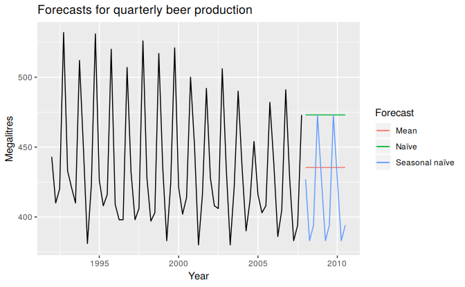

Figure 3.1: Forecasts of Australian quarterly beer production.

In Figure 3.2, the non-seasonal methods were applied to a series of 250 days of the Dow Jones Index.

# Set training data to first 250 days
dj2 <- window(dj,end=250)
# Plot some forecasts
autoplot(dj2) +
  forecast::autolayer(meanf(dj2, h=42)$mean, series="Mean") +
  forecast::autolayer(rwf(dj2, h=42)$mean, series="Naïve") +
  forecast::autolayer(rwf(dj2, drift=TRUE, h=42)$mean, series="Drift") +
  ggtitle("Dow Jones Index (daily ending 15 Jul 94)") +
  xlab("Day") + ylab("") +
  guides(colour=guide_legend(title="Forecast"))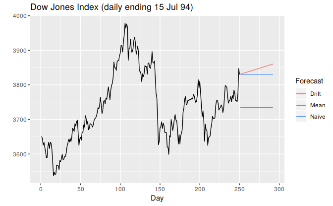

Figure 3.2: Forecasts based on 250 days of the Dow Jones Index.

Sometimes one of these simple methods will be the best forecasting method available; but in many cases, these methods will serve as benchmarks rather than the method of choice. That is, any forecasting methods we develop will be compared to these simple methods to ensure that the new method is better than these simple alternatives. If not, the new method is not worth considering.