6.5 SEATS decomposition

“SEATS” stands for “Seasonal Extraction in ARIMA Time Series” (ARIMA models are discussed in Chapter 8). This procedure was developed at the Bank of Spain, and is now widely used by government agencies around the world. The procedure works only with quarterly and monthly data. So seasonality of other kinds, such as daily data, or hourly data, or weekly data, require an alternative approach.

The details are beyond the scope of this book. However, a complete discussion of the method is available in Dagum and Bianconcini (2016). Here we will only demonstrate how to use it via the seasonal package.

library(seasonal)
elecequip %>% seas() %>%
autoplot() +
  ggtitle("SEATS decomposition of electrical equipment index")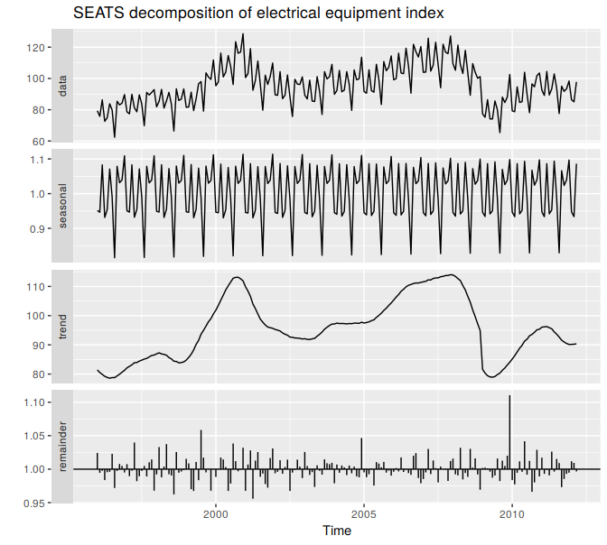

Figure 6.12: A SEATS decomposition of the new orders index for electrical equipment.

The result is quite similar to the X11 decomposition shown in Figure 6.9.

As with the X11 method, we can use the seasonal(), trendcycle() and remainder() functions to extract the individual components, and seasadj() to compute the seasonally adjusted time series.

The seasonal package has many options for handling variations of X11 and SEATS. See the package website for a detailed introduction to the options and features available.

References

Dagum, Estela Bee, and Silvia Bianconcini. 2016. Seasonal Adjustment Methods and Real Time Trend-Cycle Estimation: Springer.