7.6 Estimation and model selection
Estimating ETS models
An alternative to estimating the parameters by minimizing the sum of squared errors is to maximize the “likelihood”. The likelihood is the probability of the data arising from the specified model. Thus, a large likelihood is associated with a good model. For an additive error model, maximizing the likelihood gives the same results as minimizing the sum of squared errors. However, different results will be obtained for multiplicative error models. In this section, we will estimate the smoothing parameters \(\alpha\), \(\beta\), \(\gamma\) and \(\phi\), and the initial states \(\ell_0\), \(b_0\), \(s_0,s_{-1},\dots,s_{-m+1}\), by maximizing the likelihood.
The possible values that the smoothing parameters can take are restricted. Traditionally, the parameters have been constrained to lie between 0 and 1 so that the equations can be interpreted as weighted averages. That is, \(0< \alpha,\beta^*,\gamma^*,\phi<1\). For the state space models, we have set \(\beta=\alpha\beta^*\) and \(\gamma=(1-\alpha)\gamma^*\). Therefore, the traditional restrictions translate to \(0< \alpha <1\), \(0 < \beta < \alpha\) and \(0< \gamma < 1-\alpha\). In practice, the damping parameter \(\phi\) is usually constrained further to prevent numerical difficulties in estimating the model. In R, it is restricted so that \(0.8<\phi<0.98\).
Another way to view the parameters is through a consideration of the mathematical properties of the state space models. The parameters are constrained in order to prevent observations in the distant past having a continuing effect on current forecasts. This leads to some admissibility constraints on the parameters, which are usually (but not always) less restrictive than the usual region. For example, for the ETS(A,N,N) model, the usual parameter region is \(0< \alpha <1\) but the admissible region is \(0< \alpha <2\). For the ETS(A,A,N) model, the usual parameter region is \(0<\alpha<1\) and \(0<\beta<\alpha\) but the admissible region is \(0<\alpha<2\) and \(0<\beta<4-2\alpha\).
Model selection
A great advantage of the ETS statistical framework is that information criteria can be used for model selection. The AIC, AIC\(_{\text{c}}\) and BIC, introduced in Section 5.5, can be used here to determine which of the ETS models is most appropriate for a given time series.
For ETS models, Akaike’s Information Criterion (AIC) is defined as \[ \text{AIC} = -2\log(L) + 2k, \] where \(L\) is the likelihood of the model and \(k\) is the total number of parameters and initial states that have been estimated (including the residual variance).
The AIC corrected for small sample bias (AIC\(_\text{c}\)) is defined as \[ \text{AIC}_{\text{c}} = \text{AIC} + \frac{k(k+1)}{T-k-1}, \] and the Bayesian Information Criterion (BIC) is \[ \text{BIC} = \text{AIC} + k[\log(T)-2]. \]
Three of the combinations of (Error, Trend, Seasonal) can lead to numerical difficulties. Specifically, the models that can cause such instabilities are ETS(A,N,M), ETS(A,A,M), and ETS(A,Ad,M). We normally do not consider these particular combinations when selecting a model.
Models with multiplicative errors are useful when the data are strictly positive, but are not numerically stable when the data contain zeros or negative values. Therefore, multiplicative error models will not be considered if the time series is not strictly positive. In that case, only the six fully additive models will be applied.
The ets() function in R
The models can be estimated in R using the ets() function in the forecast package. Unlike the ses, holt and hw functions, the ets function does not produce forecasts. Rather, it estimates the model parameters and returns information about the fitted model.
The R code below shows the most important arguments that this function can take, and their default values. If only the time series is specified, and all other arguments are left at their default values, then an appropriate model will be selected automatically. We explain the arguments below. See the help file for a more complete description.
ets(y, model="ZZZ", damped=NULL, alpha=NULL, beta=NULL, gamma=NULL,
    phi=NULL, lambda=NULL, biasadj=FALSE, additive.only=FALSE,
restrict=TRUE, allow.multiplicative.trend=FALSE)y- The time series to be forecast.
model- A three-letter code indicating the model to be estimated using the ETS classification and notation. The possible inputs are “N” for none, “A” for additive, “M” for multiplicative, or “Z” for automatic selection. If any of the inputs is left as “Z”, then this component is selected according to the information criterion chosen. The default value of
ZZZensures that all components are selected using the information criterion. damped- If
damped=TRUE, then a damped trend will be used (either A or M). Ifdamped=FALSE, then a non-damped trend will used. Ifdamped=NULL(the default), then either a damped or a non-damped trend will be selected, depending on which model has the smallest value for the information criterion. alpha,beta,gamma,phi- The values of the smoothing parameters can be specified using these arguments. If they are set to
NULL(the default setting for each of them), the parameters are estimated. lambda- Box-Cox transformation parameter. It will be ignored if
lambda=NULL(the default value). Otherwise, the time series will be transformed before the model is estimated. Whenlambdais notNULL,additive.onlyis set toTRUE. biasadj- If
TRUEandlambdais notNULL, then the back-transformed fitted values and forecasts will be bias-adjusted. additive.only- Only models with additive components will be considered if
additive.only=TRUE. Otherwise, all models will be considered. restrict- If
restrict=TRUE(the default), the models that cause numerical difficulties are not considered in model selection. allow.multiplicative.trend- Multiplicative trend models are also available, but not covered in this book. Set this argument to
TRUEto allow these models to be considered.
Working with ets objects
The ets() function will return an object of class ets. There are many R functions designed to make working with ets objects easy. A few of them are described below.
coef()- returns all fitted parameters.
accuracy()- returns accuracy measures computed on the training data.
summary()- prints some summary information about the fitted model.
autoplot()andplot()- produce time plots of the components.
residuals()- returns residuals from the estimated model.
fitted()- returns one-step forecasts for the training data.
simulate()- will simulate future sample paths from the fitted model.
forecast()- computes point forecasts and prediction intervals, as described in the next section.
Example: International tourist visitor nights in Australia
We now employ the ETS statistical framework to forecast tourist visitor nights in Australia by international arrivals over the period 2016–2019. We let the ets() function select the model by minimizing the AICc.
aust <- window(austourists, start=2005)
fit <- ets(aust)
summary(fit)
#> ETS(M,A,M)
#>
#> Call:
#>  ets(y = aust)
#>
#>   Smoothing parameters:
#>     alpha = 0.1908
#>     beta  = 0.0392
#>     gamma = 2e-04
#>
#>   Initial states:
#>     l = 32.3679
#>     b = 0.9281
#>     s = 1.02 0.963 0.768 1.25
#>
#>   sigma:  0.0383
#>
#>  AIC AICc  BIC
#>  225  230  241
#>
#> Training set error measures:
#>                  ME RMSE  MAE    MPE MAPE  MASE  ACF1
#> Training set 0.0484 1.67 1.25 -0.185 2.69 0.409 0.201
The model selected is ETS(M,A,M):
\[\begin{align*} y_{t} &= (\ell_{t-1} + b_{t-1})s_{t-m}(1 + \varepsilon_t)\\ \ell_t &= (\ell_{t-1} + b_{t-1})(1 + \alpha \varepsilon_t)\\ b_t &=b_{t-1} + \beta(\ell_{t-1} + b_{t_1})\varepsilon_t\\ s_t &= s_{t-m}(1+ \gamma \varepsilon_t). \end{align*}\]
The parameter estimates are \(\alpha=0.1908\), \(\beta=0.03919\), and \(\gamma=0.0001917\). The output also returns the estimates for the initial states \(\ell_0\), \(b_0\), \(s_{0}\), \(s_{-1}\), \(s_{-2}\) and \(s_{-3}.\) Compare these with the values obtained for the Holt-Winters method with multiplicative seasonality presented in Table 7.5. Although this model gives equivalent point forecasts to a multiplicative Holt-Winters’ method, the parameters have been estimated differently. With the ets() function, the default estimation method is maximum likelihood rather than minimum sum of squares.
Figure 7.9 shows the states over time, while Figure 7.11 shows point forecasts and prediction intervals generated from the model. The small values of \(\beta\) and \(\gamma\) mean that the slope and seasonal components change very little over time. The narrow prediction intervals indicate that the series is relatively easy to forecast due to the strong trend and seasonality.
autoplot(fit)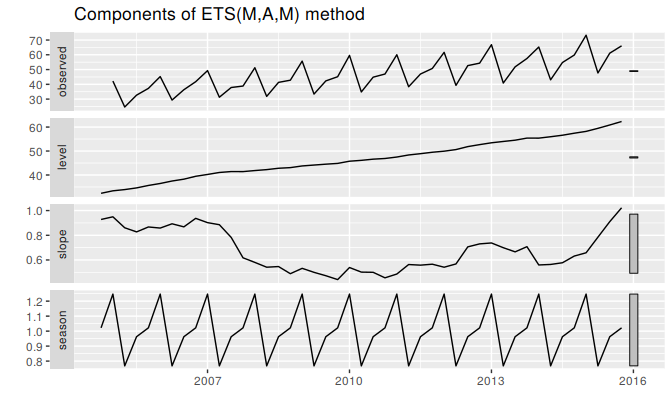
Figure 7.9: Graphical representation of the estimated states over time.
Because this model has multiplicative errors, the residuals are not equivalent to the one-step forecast errors. The residuals are given by \(\hat{\varepsilon}_t\), while the one-step forecast errors are defined as \(y_t - \hat{y}_{t|t-1}\). We can obtain both using the residuals function.
cbind('Residuals' = residuals(fit),
      'Forecast errors' = residuals(fit, type='response')) %>%
  autoplot(facet=TRUE) + xlab("Year") + ylab("")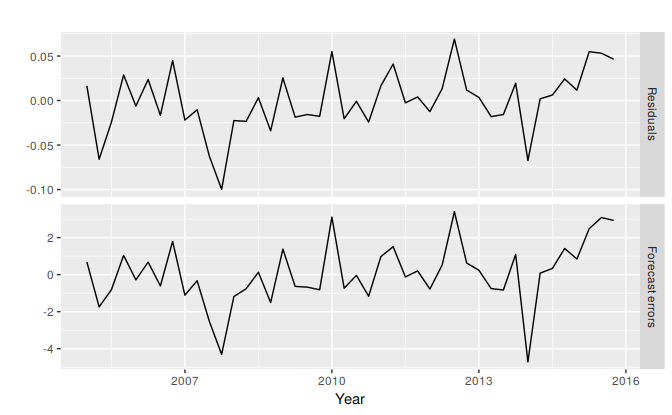
Figure 7.10: Residuals and one-step forecast errors from the ETS(M,A,M) model.
The type argument is used in the residuals function to distinguish between residuals and forecast errors. The default is type='innovation' which gives regular residuals.