6.2 Moving averages
The classical method of time series decomposition originated in the 1920s and was widely used until the 1950s. It still forms the basis of many time series decomposition methods, so it is important to understand how it works. The first step in a classical decomposition is to use a moving average method to estimate the trend-cycle, so we begin by discussing moving averages.
Moving average smoothing
A moving average of order \(m\) can be written as \[ \hat{T}_{t} = \frac{1}{m} \sum_{j=-k}^k y_{t+j}, \] where \(m=2k+1\). That is, the estimate of the trend-cycle at time \(t\) is obtained by averaging values of the time series within \(k\) periods of \(t\). Observations that are nearby in time are also likely to be close in value, and the average eliminates some of the randomness in the data, leaving a smooth trend-cycle component. We call this an “\(m\)-MA”, meaning a moving average of order \(m\).
autoplot(elecsales) + xlab("Year") + ylab("GWh") +
  ggtitle("Annual electricity sales: South Australia")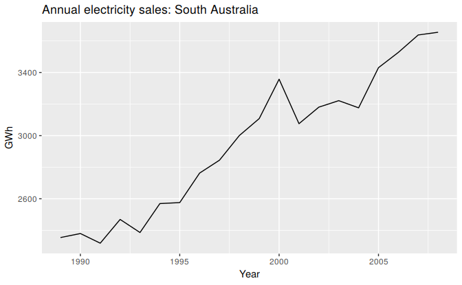
Figure 6.4: Residential electricity sales (excluding hot water) for South Australia: 1989–2008.
For example, consider Figure 6.4 which shows the volume of electricity sold to residential customers in South Australia each year from 1989 to 2008 (hot water sales have been excluded). The data are also shown in Table 6.1.
ma5 <- ma(elecsales, 5)| Year | Sales (GWh) | 5-MA |
|---|---|---|
| 1989 | 2354.34 | |
| 1990 | 2379.71 | |
| 1991 | 2318.52 | 2381.53 |
| 1992 | 2468.99 | 2424.56 |
| 1993 | 2386.09 | 2463.76 |
| 1994 | 2569.47 | 2552.60 |
| 1995 | 2575.72 | 2627.70 |
| 1996 | 2762.72 | 2750.62 |
| 1997 | 2844.50 | 2858.35 |
| 1998 | 3000.70 | 3014.70 |
| 1999 | 3108.10 | 3077.30 |
| 2000 | 3357.50 | 3144.52 |
| 2001 | 3075.70 | 3188.70 |
| 2002 | 3180.60 | 3202.32 |
| 2003 | 3221.60 | 3216.94 |
| 2004 | 3176.20 | 3307.30 |
| 2005 | 3430.60 | 3398.75 |
| 2006 | 3527.48 | 3485.43 |
| 2007 | 3637.89 | |
| 2008 | 3655.00 |
In the second column of this table, a moving average of order 5 is shown, providing an estimate of the trend-cycle. The first value in this column is the average of the first five observations (1989–1993); the second value in the 5-MA column is the average of the values for 1990–1994; and so on. Each value in the 5-MA column is the average of the observations in the five year period centered on the corresponding year. There are no values for either the first two years or the last two years, because we do not have two observations on either side. In the formula above, column 5-MA contains the values of \(\hat{T}_{t}\) with \(k=2\). To see what the trend-cycle estimate looks like, we plot it along with the original data in Figure 6.5.
autoplot(elecsales, series="Data") +
  forecast::autolayer(ma(elecsales,5), series="5-MA") +
  xlab("Year") + ylab("GWh") +
  ggtitle("Annual electricity sales: South Australia") +
  scale_colour_manual(values=c("Data"="grey50","5-MA"="red"),
                     breaks=c("Data","5-MA"))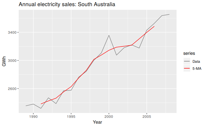
Figure 6.5: Residential electricity sales (black) along with the 5-MA estimate of the trend-cycle (red).
Notice that the trend-cycle (in red) is smoother than the original data and captures the main movement of the time series without all of the minor fluctuations. The moving average method does not allow estimates of \(T_{t}\) when \(t\) is close to the ends of the series; hence the red line does not extend to the edges of the graph on either side. Later we will use more sophisticated methods of trend-cycle estimation which do allow estimates near the endpoints.
The order of the moving average determines the smoothness of the trend-cycle estimate. In general, a larger order means a smoother curve. Figure 6.6 shows the effect of changing the order of the moving average for the residential electricity sales data.
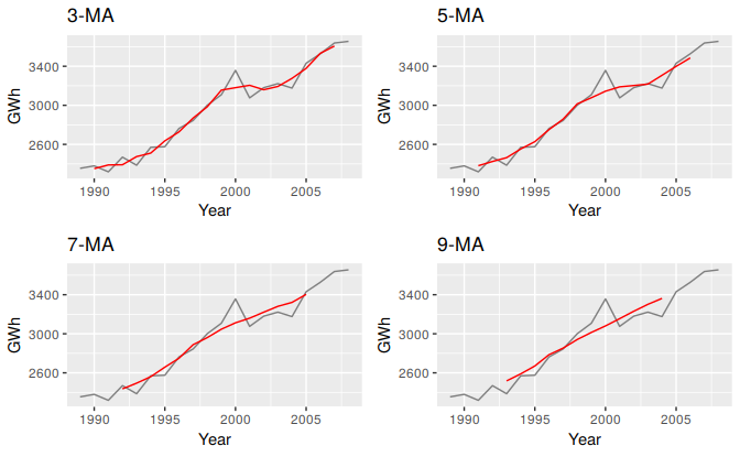
Figure 6.6: Different moving averages applied to the residential electricity sales data.
Simple moving averages such as these are usually of an odd order (e.g., 3, 5, 7, etc.) This is so they are symmetric: in a moving average of order \(m=2k+1\), there are \(k\) earlier observations, \(k\) later observations and the middle observation that are averaged. But if \(m\) was even, it would no longer be symmetric.
Moving averages of moving averages
It is possible to apply a moving average to a moving average. One reason for doing this is to make an even-order moving average symmetric.
For example, we might take a moving average of order 4, and then apply another moving average of order 2 to the results. In the following table, this has been done for the first few years of the Australian quarterly beer production data.
beer2 <- window(ausbeer,start=1992)
ma4 <- ma(beer2, order=4, centre=FALSE)
ma2x4 <- ma(beer2, order=4, centre=TRUE)| Year | Quarter | Observation | 4-MA | 2x4-MA |
|---|---|---|---|---|
| 1992 | Q1 | 443 | ||
| 1992 | Q2 | 410 | 451 | |
| 1992 | Q3 | 420 | 449 | 450 |
| 1992 | Q4 | 532 | 452 | 450 |
| 1993 | Q1 | 433 | 449 | 450 |
| 1993 | Q2 | 421 | 444 | 446 |
| 1993 | Q3 | 410 | 448 | 446 |
| 1993 | Q4 | 512 | 438 | 443 |
| 1994 | Q1 | 449 | 441 | 440 |
| 1994 | Q2 | 381 | 446 | 444 |
| 1994 | Q3 | 423 | 440 | 443 |
| 1994 | Q4 | 531 | 447 | 444 |
| 1995 | Q1 | 426 | 445 | 446 |
| 1995 | Q2 | 408 | 442 | 444 |
| 1995 | Q3 | 416 | 438 | 440 |
| 1995 | Q4 | 520 | 436 | 437 |
| 1996 | Q1 | 409 | 431 | 434 |
| 1996 | Q2 | 398 | 428 | 430 |
| 1996 | Q3 | 398 | 434 | 431 |
| 1996 | Q4 | 507 | 434 | 434 |
The notation “\(2\times4\)-MA” in the last column means a 4-MA followed by a 2-MA. The values in the last column are obtained by taking a moving average of order 2 of the values in the previous column. For example, the first two values in the 4-MA column are 451.25=(443+410+420+532)/4 and 448.75=(410+420+532+433)/4. The first value in the 2x4-MA column is the average of these two: 450.00=(451.25+448.75)/2.
When a 2-MA follows a moving average of an even order (such as 4), it is called a “centered moving average of order 4”. This is because the results are now symmetric. To see that this is the case, we can write the \(2\times4\)-MA as follows: \[\begin{align*} \hat{T}_{t} &= \frac{1}{2}\Big[ \frac{1}{4} (y_{t-2}+y_{t-1}+y_{t}+y_{t+1}) + \frac{1}{4} (y_{t-1}+y_{t}+y_{t+1}+y_{t+2})\Big] \\ &= \frac{1}{8}y_{t-2}+\frac14y_{t-1} + \frac14y_{t}+\frac14y_{t+1}+\frac18y_{t+2}. \end{align*}\] It is now a weighted average of observations, but it is symmetric.
Other combinations of moving averages are also possible. For example, a \(3\times3\)-MA is often used, and consists of a moving average of order 3 followed by another moving average of order 3. In general, an even order MA should be followed by an even order MA to make it symmetric. Similarly, an odd order MA should be followed by an odd order MA.
Estimating the trend-cycle with seasonal data
The most common use of centered moving averages is in estimating the trend-cycle from seasonal data. Consider the \(2\times4\)-MA: \[ \hat{T}_{t} = \frac{1}{8}y_{t-2} + \frac14y_{t-1} + \frac14y_{t} + \frac14y_{t+1} + \frac18y_{t+2}. \] When applied to quarterly data, each quarter of the year is given equal weight as the first and last terms apply to the same quarter in consecutive years. Consequently, the seasonal variation will be averaged out and the resulting values of \(\hat{T}_t\) will have little or no seasonal variation remaining. A similar effect would be obtained using a \(2\times 8\)-MA or a \(2\times 12\)-MA to quarterly data.
In general, a \(2\times m\)-MA is equivalent to a weighted moving average of order \(m+1\) where all observations take the weight \(1/m\), except for the first and last terms which take weights \(1/(2m)\). So, if the seasonal period is even and of order \(m\), use a \(2\times m\)-MA to estimate the trend-cycle. If the seasonal period is odd and of order \(m\), use a \(m\)-MA to estimate the trend-cycle. For example, a \(2\times 12\)-MA can be used to estimate the trend-cycle of monthly data and a 7-MA can be used to estimate the trend-cycle of daily data with a weekly seasonality.
Other choices for the order of the MA will usually result in trend-cycle estimates being contaminated by the seasonality in the data.
###Example: Electrical equipment manufacturing {-}
autoplot(elecequip, series="Data") +
  forecast::autolayer(ma(elecequip, 12), series="12-MA") +
  xlab("Year") + ylab("New orders index") +
  ggtitle("Electrical equipment manufacturing (Euro area)") +
  scale_colour_manual(values=c("Data"="grey","12-MA"="red"),
    breaks=c("Data","12-MA"))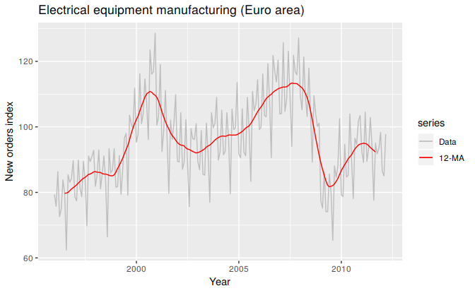
Figure 6.7: A 2x12-MA applied to the electrical equipment orders index.
Figure 6.7 shows a \(2\times12\)-MA applied to the electrical equipment orders index. Notice that the smooth line shows no seasonality; it is almost the same as the trend-cycle shown in Figure 6.1, which was estimated using a much more sophisticated method than moving averages. Any other choice for the order of the moving average (except for 24, 36, etc.) would have resulted in a smooth line that showed some seasonal fluctuations.
Weighted moving averages
Combinations of moving averages result in weighted moving averages. For example, the \(2\times4\)-MA discussed above is equivalent to a weighted 5-MA with weights given by \(\left[\frac{1}{8},\frac{1}{4},\frac{1}{4},\frac{1}{4},\frac{1}{8}\right]\). In general, a weighted \(m\)-MA can be written as \[ \hat{T}_t = \sum_{j=-k}^k a_j y_{t+j}, \] where \(k=(m-1)/2\), and the weights are given by \(\left[a_{-k},\dots,a_k\right]\). It is important that the weights all sum to one and that they are symmetric so that \(a_j = a_{-j}\). The simple \(m\)-MA is a special case where all of the weights are equal to \(1/m\).
A major advantage of weighted moving averages is that they yield a smoother estimate of the trend-cycle. Instead of observations entering and leaving the calculation at full weight, their weights slowly increase and then slowly decrease, resulting in a smoother curve.
Some specific sets of weights are widely used due to their mathematical properties. Some of these are given in Table 6.3.
| \(a_{0}\) | \(a_{1}\) | \(a_{2}\) | \(a_{3}\) | \(a_{4}\) | \(a_{5}\) | \(a_{6}\) | \(a_{7}\) | \(a_{8}\) | \(a_{9}\) | \(a_{10}\) | \(a_{11}\) | |
|---|---|---|---|---|---|---|---|---|---|---|---|---|
| 3-MA | 0.333 | 0.333 | ||||||||||
| 5-MA | 0.200 | 0.200 | 0.200 | |||||||||
| 2x12-MA | 0.083 | 0.083 | 0.083 | 0.083 | 0.083 | 0.083 | 0.042 | |||||
| 3x3-MA | 0.333 | 0.222 | 0.111 | |||||||||
| 3x5-MA | 0.200 | 0.200 | 0.133 | 0.067 | ||||||||
| S15-MA | 0.231 | 0.209 | 0.144 | 0.066 | 0.009 | -0.016 | -0.019 | -0.009 | ||||
| S21-MA | 0.171 | 0.163 | 0.134 | 0.094 | 0.051 | 0.017 | -0.006 | -0.014 | -0.014 | -0.009 | -0.003 | |
| H5-MA | 0.558 | 0.294 | -0.073 | |||||||||
| H9-MA | 0.330 | 0.267 | 0.119 | -0.010 | -0.041 | |||||||
| H13-MA | 0.240 | 0.214 | 0.147 | 0.066 | 0.000 | -0.028 | -0.019 | |||||
| H23-MA | 0.148 | 0.138 | 0.122 | 0.097 | 0.068 | 0.039 | 0.013 | -0.005 | -0.015 | -0.016 | -0.011 | -0.004 |