6.6 STL decomposition
STL is a very versatile and robust method for decomposing time series. STL is an acronym for “Seasonal and Trend decomposition using Loess”, while Loess is a method for estimating nonlinear relationships. The STL method was developed by Cleveland et al. (1990).
STL has several advantages over the classical, SEATS and X-11 decomposition methods:
Unlike SEATS and X-11, STL will handle any type of seasonality, not only monthly and quarterly data.
The seasonal component is allowed to change over time, and the rate of change can be controlled by the user.
The smoothness of the trend-cycle can also be controlled by the user.
It can be robust to outliers (i.e., the user can specify a robust decomposition), so that occasional unusual observations will not affect the estimates of the trend-cycle and seasonal components. They will, however, affect the remainder component.
On the other hand, STL has some disadvantages. In particular, it does not handle trading day or calendar variation automatically, and it only provides facilities for additive decompositions.
It is possible to obtain a multiplicative decomposition by first taking logs of the data, then back-transforming the components. Decompositions between additive and multiplicative can be obtained using a Box-Cox transformation of the data with \(0<\lambda<1\). A value of \(\lambda=0\) corresponds to the multiplicative decomposition while \(\lambda=1\) is equivalent to an additive decomposition.
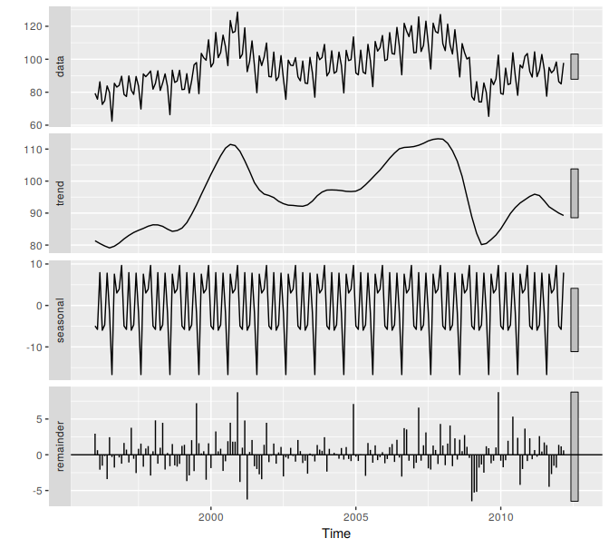
The best way to begin learning how to use STL is to see some examples and experiment with the settings. Figure 6.2 showed an example of STL applied to the electrical equipment orders data. Figure 6.13 shows an alternative STL decomposition where the trend-cycle is more flexible, the seasonal component does not change over time, and the robust option has been used. Here, it is more obvious that there has been a down-turn at the end of the series, and that the orders in 2009 were unusually low (corresponding to some large negative values in the remainder component).
elecequip %>%
  stl(t.window=13, s.window="periodic", robust=TRUE) %>%
  autoplot
Figure 6.13: The electrical equipment orders (top) and its three additive components obtained from a robust STL decomposition with flexible trend-cycle and fixed seasonality.
The two main parameters to be chosen when using STL are the trend-cycle window (t.window) and the seasonal window (s.window). These control how rapidly the trend-cycle and seasonal components can change. Smaller values allow for more rapid changes. Both t.window and s.window should be odd numbers and refer to the number of consecutive years to be used when estimating the trend-cycle and seasonal components respectively. The user must specify s.window as there is no default. Setting it to to be infinite is equivalent to forcing the seasonal component to be periodic (i.e., identical across years). Specifying t.window is optional, and a default value will be used if it is omitted.
As with the other decomposition methods discussed in this book, to obtain the separate components plotted in Figure 6.8, use the seasonal() function for the seasonal component, the trendcycle() function for trend-cycle component, and the remainder() function for the remainder component. The seasadj() function can be used to compute the seasonally adjusted series.
References
Cleveland, Robert B, William S Cleveland, Jean E McRae, and Irma J Terpenning. 1990. “STL: A Seasonal-Trend Decomposition Procedure Based on Loess.” Journal of Official Statistics 6 (1): 3–73.