7.1 Simple exponential smoothing

The simplest of the exponentially smoothing methods is naturally called “simple exponential smoothing” (SES)¹². This method is suitable for forecasting data with no clear trend or seasonal pattern. For example, the data in Figure 7.1 do not display any clear trending behaviour or any seasonality. (There is a rise in the last few years, which might suggest a trend. We will consider whether a trended method would be better for this series later in this chapter.) We have already considered the naïve and the average as possible methods for forecasting such data (Section 3.1).

oildata <- window(oil, start=1996)
autoplot(oildata) +
  ylab("Oil (millions of tonnes)") + xlab("Year")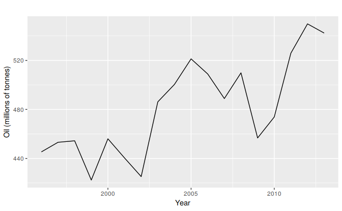

Figure 7.1: Oil production in Saudi Arabia from 1980 to 2013.

Using the naïve method, all forecasts for the future are equal to the last observed value of the series, $$\hat{y}_{T+h|T} = y_{T},$$ for $h=1,2,\dots$. Hence, the naïve method assumes that the most recent observation is the only important one, and all previous observations provide no information for the future. This can be thought of as a weighted average where all of the weight is given to the last observation.

Using the average method, all future forecasts are equal to a simple average of the observed data, $$\hat{y}_{T+h|T} = \frac1T \sum_{t=1}^T y_t,$$ for $h=1,2,\dots$. Hence, the average method assumes that all observations are of equal importance, and gives them equal weights when generating forecasts.

We often want something between these two extremes. For example, it may be sensible to attach larger weights to more recent observations than to observations from the distant past. This is exactly the concept behind simple exponential smoothing. Forecasts are calculated using weighted averages, where the weights decrease exponentially as observations come from further in the past — the smallest weights are associated with the oldest observations: $$\begin{equation} \hat{y}_{T+1|T} = \alpha y_T + \alpha(1-\alpha) y_{T-1} + \alpha(1-\alpha)^2 y_{T-2}+ \alpha(1-\alpha)^3 y_{T-3}+\cdots, \tag{7.1} \end{equation}$$ where $0 \le \alpha \le 1$ is the smoothing parameter. The one-step-ahead forecast for time $T+1$ is a weighted average of all of the observations in the series $y_1,\dots,y_T$. The rate at which the weights decrease is controlled by the parameter $\alpha$.

Table 7.1 shows the weights attached to observations for four different values of $\alpha$ when forecasting using simple exponential smoothing. Note that the sum of the weights even for a small value of $\alpha$ will be approximately one for any reasonable sample size.

Table 7.1: Exponentially decaying weights attached to observations of the time series when generating forecasts using simple exponential smoothing.

	$\alpha=0.2$	$\alpha=0.4$	$\alpha=0.6$	$\alpha=0.8$
$y_{T}$	0.2000	0.4000	0.6000	0.8000
$y_{T-1}$	0.1600	0.2400	0.2400	0.1600
$y_{T-2}$	0.1280	0.1440	0.0960	0.0320
$y_{T-3}$	0.1024	0.0864	0.0384	0.0064
$y_{T-4}$	0.0819	0.0518	0.0154	0.0013
$y_{T-5}$	0.0655	0.0311	0.0061	0.0003

For any $\alpha$ between 0 and 1, the weights attached to the observations decrease exponentially as we go back in time, hence the name “exponential smoothing”. If $\alpha$ is small (i.e., close to 0), more weight is given to observations from the more distant past. If $\alpha$ is large (i.e., close to 1), more weight is given to the more recent observations. For the extreme case where $\alpha=1$, $\hat{y}_{T+1|T}=y_T$, and the forecasts are equal to the naïve forecasts.

We present two equivalent forms of simple exponential smoothing, each of which leads to the forecast equation (7.1).

Weighted average form

The forecast at time $t+1$ is equal to a weighted average between the most recent observation $y_t$ and the most recent forecast $\hat{y}_{t|t-1}$, $$\hat{y}_{t+1|t} = \alpha y_t + (1-\alpha) \hat{y}_{t|t-1}$$ for $t=1,\dots,T$, where $0 \le \alpha \le 1$ is the smoothing parameter.

The process has to start somewhere, so we let the first forecast of $y_1$ be denoted by $\ell_0$ (which we will have to estimate). Then $$\begin{align*} \hat{y}_{2|1} &= \alpha y_1 + (1-\alpha) \ell_0\\ \hat{y}_{3|2} &= \alpha y_2 + (1-\alpha) \hat{y}_{2|1}\\ \hat{y}_{4|3} &= \alpha y_3 + (1-\alpha) \hat{y}_{3|2}\\ \vdots\\ \hat{y}_{T+1|T} &= \alpha y_T + (1-\alpha) \hat{y}_{T|T-1}. \end{align*}$$ Substituting each equation into the following equation, we obtain $$\begin{align*} \hat{y}_{3|2} & = \alpha y_2 + (1-\alpha) \left[\alpha y_1 + (1-\alpha) \ell_0\right] \\ & = \alpha y_2 + \alpha(1-\alpha) y_1 + (1-\alpha)^2 \ell_0 \\ \hat{y}_{4|3} & = \alpha y_3 + (1-\alpha) [\alpha y_2 + \alpha(1-\alpha) y_1 + (1-\alpha)^2 \ell_0]\\ & = \alpha y_3 + \alpha(1-\alpha) y_2 + \alpha(1-\alpha)^2 y_1 + (1-\alpha)^3 \ell_0 \\ & ~~\vdots \\ \hat{y}_{T+1|T} & = \sum_{j=0}^{T-1} \alpha(1-\alpha)^j y_{T-j} + (1-\alpha)^T \ell_{0}. \end{align*}$$ The last term becomes tiny for large $T$. So, the weighted average form leads to the same forecast equation (7.1).

Component form

An alternative representation is the component form. For simple exponential smoothing, the only component included is the level, $\ell_t$. (Other methods which are considered later in this chapter may also include a trend $b_t$ and a seasonal component $s_t$.) Component form representations of exponential smoothing methods comprise a forecast equation and a smoothing equation for each of the components included in the method. The component form of simple exponential smoothing is given by: $$\begin{align*} \text{Forecast equation} && \hat{y}_{t+1|t} & = \ell_{t}\\ \text{Smoothing equation} && \ell_{t} & = \alpha y_{t} + (1 - \alpha)\ell_{t-1}, \end{align*}$$ where $\ell_{t}$ is the level (or the smoothed value) of the series at time $t$. The forecast equation shows that the forecast value at time $t+1$ is the estimated level at time $t$. The smoothing equation for the level (usually referred to as the level equation) gives the estimated level of the series at each period $t$.

Applying the forecast equation for time $T$ gives $\hat{y}_{T+1|T} = \ell_{T}$, the most recent estimated level.

If we replace $\ell_t$ with $\hat{y}_{t+1|t}$ and $\ell_{t-1}$ with $\hat{y}_{t|t-1}$ in the smoothing equation, we will recover the weighted average form of simple exponential smoothing.

The component form of simple exponential smoothing is not particularly useful, but it will be the easiest form to use when we start adding other components.

Multi-horizon Forecasts

So far, we have only given forecast equations for one step ahead. Simple exponential smoothing has a “flat” forecast function, and therefore for longer forecast horizons, $$\hat{y}_{T+h|T} = \hat{y}_{T+1|T}=\ell_T, \qquad h=2,3,\dots.$$ Remember that these forecasts will only be suitable if the time series has no trend or seasonal component.

Optimization

The application of every exponential smoothing method requires the smoothing parameters and the initial values to be chosen. In particular, for simple exponential smoothing, we need to select the values of $\alpha$ and $\ell_0$. All forecasts can be computed from the data once we know those values. For the methods that follow there is usually more than one smoothing parameter and more than one initial component to be chosen.

In some cases, the smoothing parameters may be chosen in a subjective manner — the forecaster specifies the value of the smoothing parameters based on previous experience. However, a more reliable and objective way to obtain values for the unknown parameters is to estimate them from the observed data.

In Section 5.2, we estimated the coefficients of a regression model by minimizing the sum of the squared errors (SSE). Similarly, the unknown parameters and the initial values for any exponential smoothing method can be estimated by minimizing the SSE. The errors are specified as $e_t=y_t - \hat{y}_{t|t-1}$ for $t=1,\dots,T$ (the one-step-ahead training errors). Hence, we find the values of the unknown parameters and the initial values that minimize $$\begin{equation} \text{SSE}=\sum_{t=1}^T(y_t - \hat{y}_{t|t-1})^2=\sum_{t=1}^Te_t^2. \tag{7.2} \end{equation}$$

Unlike the regression case (where we have formulas which return the values of the regression coefficients that minimize the SSE), this involves a non-linear minimization problem, and we need to use an optimization tool to solve it.

Example: Oil production

In this example, simple exponential smoothing is applied to forecast oil production in Saudi Arabia.

oildata <- window(oil, start=1996)
# Estimate parameters
fc <- ses(oildata, h=5)
# Accuracy of one-step-ahead training errors over period 1--12
round(accuracy(fc),2)
#>               ME RMSE  MAE MPE MAPE MASE  ACF1
#> Training set 6.4 28.1 22.3 1.1 4.61 0.93 -0.03

This gives parameters $\alpha=0.83$ and $\ell_0=446.6$, obtained by minimizing SSE (equivalently RMSE) over periods $t=1,2,\dots,12$, subject to the restriction that $0\le\alpha\le1$.

In Table 7.2 we demonstrate the calculation using these parameters. The second last column shows the estimated level for times $t=0$ to $t=12$; the last few rows of the last column show the forecasts for $h=1,2,3$.

Table 7.2: Forecasting the total oil production in millions of tonnes for Saudi Arabia using simple exponential smoothing.

Year	Time	Observation	Level	Forecast
	$t$	$y_t$	$\ell_t$	$\hat{y}_{t+1|t}$
1995	0		446.59
1996	1	445.36	445.57	446.59
1997	2	453.20	451.93	445.57
1998	3	454.41	454.00	451.93
1999	4	422.38	427.63	454.00
2000	5	456.04	451.32	427.63
2001	6	440.39	442.20	451.32
2002	7	425.19	428.02	442.20
2003	8	486.21	476.54	428.02
2004	9	500.43	496.46	476.54
2005	10	521.28	517.15	496.46
2006	11	508.95	510.31	517.15
2007	12	488.89	492.45	510.31
2008	13	509.87	506.98	492.45
2009	14	456.72	465.07	506.98
2010	15	473.82	472.36	465.07
2011	16	525.95	517.05	472.36
2012	17	549.83	544.39	517.05
2013	18	542.34	542.68	544.39
	$h$			$\hat{y}_{T+h|T}$
2014	1			542.68
2015	2			542.68
2016	3			542.68

The black line in Figure 7.2 is a plot of the data, which shows a changing level over time.

autoplot(fc) +
  forecast::autolayer(fitted(fc), series="Fitted") +
  ylab("Oil (millions of tonnes)") + xlab("Year")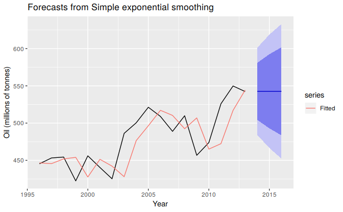

Figure 7.2: Simple exponential smoothing applied to oil production in Saudi Arabia (1996–2013).

The forecasts for the period 2014–2018 are plotted in Figure 7.2. Also plotted are one-step-ahead fitted values alongside the data over the period 1996–2013. The large value of $\alpha$ in this example is reflected in the large adjustment that takes place in the estimated level $\ell_t$ at each time. A smaller value of $\alpha$ would lead to smaller changes over time, and so the series of fitted values would be smoother.

The prediction intervals shown here are calculated using the methods described in Section 7.5. The prediction intervals show that there is considerable uncertainty in the future values of oil production over the five-year forecast period. So interpreting the point forecasts without accounting for the large uncertainty can be very misleading.

---

12. In some books it is called single exponential smoothing’’↩