8.1 Stationarity and differencing

A stationary time series is one whose properties do not depend on the time at which the series is observed.¹⁴ Thus, time series with trends, or with seasonality, are not stationary — the trend and seasonality will affect the value of the time series at different times. On the other hand, a white noise series is stationary — it does not matter when you observe it, it should look much the same at any point in time.

Some cases can be confusing — a time series with cyclic behaviour (but with no trend or seasonality) is stationary. This is because the cycles are not of a fixed length, so before we observe the series we cannot be sure where the peaks and troughs of the cycles will be.

In general, a stationary time series will have no predictable patterns in the long-term. Time plots will show the series to be roughly horizontal (although some cyclic behaviour is possible), with constant variance.

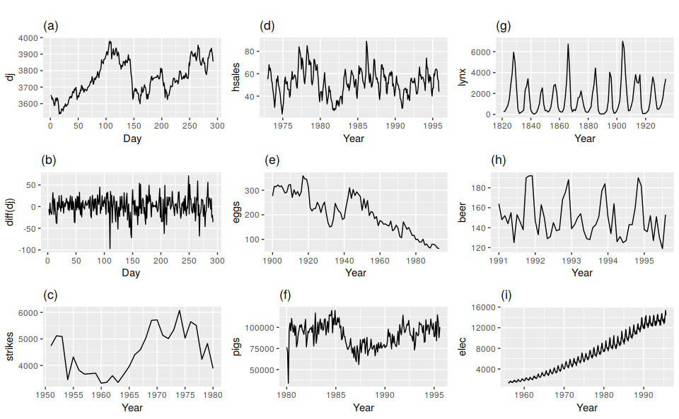
Figure 8.1: Which of these series are stationary? (a) Dow Jones index on 292 consecutive days; (b) Daily change in the Dow Jones index on 292 consecutive days; (c) Annual number of strikes in the US; (d) Monthly sales of new one-family houses sold in the US; (e) Annual price of a dozen eggs in the US (constant dollars); (f) Monthly total of pigs slaughtered in Victoria, Australia; (g) Annual total of lynx trapped in the McKenzie River district of north-west Canada; (h) Monthly Australian beer production; (i) Monthly Australian electricity production.

Consider the nine series plotted in Figure 8.1. Which of these do you think are stationary?

Obvious seasonality rules out series (d), (h) and (i). Trend rules out series (a), (c), (e), (f) and (i). Increasing variance also rules out (i). That leaves only (b) and (g) as stationary series.

At first glance, the strong cycles in series (g) might appear to make it non-stationary. But these cycles are aperiodic — they are caused when the lynx population becomes too large for the available feed, so that they stop breeding and the population falls to very low numbers, then the regeneration of their food sources allows the population to grow again, and so on. In the long-term, the timing of these cycles is not predictable. Hence the series is stationary.

Differencing

In Figure 8.1, note that the Dow Jones index was non-stationary in panel (a), but the daily changes were stationary in panel (b). This shows one way to make a time series stationary — compute the differences between consecutive observations. This is known as differencing.

Transformations such as logarithms can help to stabilize the variance of a time series. Differencing can help stabilize the mean of a time series by removing changes in the level of a time series, and therefore eliminating (or reducing) trend and seasonality.

As well as looking at the time plot of the data, the ACF plot is also useful for identifying non-stationary time series. For a stationary time series, the ACF will drop to zero relatively quickly, while the ACF of non-stationary data decreases slowly. Also, for non-stationary data, the value of \(r_1\) is often large and positive.

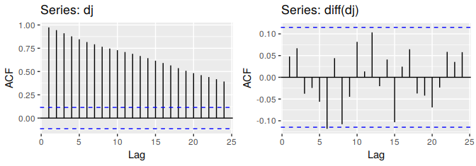
Figure 8.2: The ACF of the Dow-Jones index (left) and of the daily changes in the Dow-Jones index (right).

Box.test(diff(dj), lag=10, type="Ljung-Box")
#> 
#>  Box-Ljung test
#> 
#> data:  diff(dj)
#> X-squared = 14, df = 10, p-value = 0.2

The ACF of the differenced Dow-Jones index looks just like that of a white noise series. There is only one autocorrelation lying just outside the 95% limits, and the Ljung-Box \(Q^*\) statistic has a p-value of 0.153 (for \(h=10\)). This suggests that the daily change in the Dow-Jones index is essentially a random amount which is uncorrelated with that of previous days.

Random walk model

The differenced series is the change between consecutive observations in the original series, and can be written as \[ y'_t = y_t - y_{t-1}. \] The differenced series will have only \(T-1\) values, since it is not possible to calculate a difference \(y_1'\) for the first observation.

When the differenced series is white noise, the model for the original series can be written as \[ y_t - y_{t-1} = e_t \quad\text{or}\quad {y_t = y_{t-1} + e_t}\: . \] Random walk models are very widely used for non-stationary data, particularly financial and economic data. Random walks typically have:

• long periods of apparent trends up or down
• sudden and unpredictable changes in direction.

The forecasts from a random walk model are equal to the last observation, as future movements are unpredictable, and are equally likely to be up or down. Thus, the random walk model underpins naïve forecasts.

A closely related model allows the differences to have a non-zero mean. Then \[ y_t - y_{t-1} = c + e_t\quad\text{or}\quad {y_t = c + y_{t-1} + e_t}\: . \] The value of \(c\) is the average of the changes between consecutive observations. If \(c\) is positive, then the average change is an increase in the value of \(y_t\). Thus, \(y_t\) will tend to drift upwards. However, if \(c\) is negative, \(y_t\) will tend to drift downwards.

This is the model behind the drift method discussed in Section 3.1.

Second-order differencing

Occasionally the differenced data will not appear to be stationary and it may be necessary to difference the data a second time to obtain a stationary series: \[\begin{align*} y''_{t} &= y'_{t} - y'_{t - 1} \\ &= (y_t - y_{t-1}) - (y_{t-1}-y_{t-2})\\ &= y_t - 2y_{t-1} +y_{t-2}. \end{align*}\] In this case, \(y_t''\) will have \(T-2\) values. Then, we would model the “change in the changes” of the original data. In practice, it is almost never necessary to go beyond second-order differences.

Seasonal differencing

A seasonal difference is the difference between an observation and the corresponding observation from the previous year. So \[ y’_t = y_t - y_{t-m}, \] where \(m=\) the number of seasons. These are also called “lag-\(m\) differences”, as we subtract the observation after a lag of \(m\) periods.

If seasonally differenced data appear to be white noise, then an appropriate model for the original data is \[ y_t = y_{t-m}+e_t. \] Forecasts from this model are equal to the last observation from the relevant season. That is, this model gives seasonal naïve forecasts.

cbind("Sales ($million)" = a10,
      "Monthly log sales" = log(a10),
      "Annual change in log sales" = diff(log(a10),12)) %>%
  autoplot(facets=TRUE) +
    xlab("Year") + ylab("") +
    ggtitle("Antidiabetic drug sales")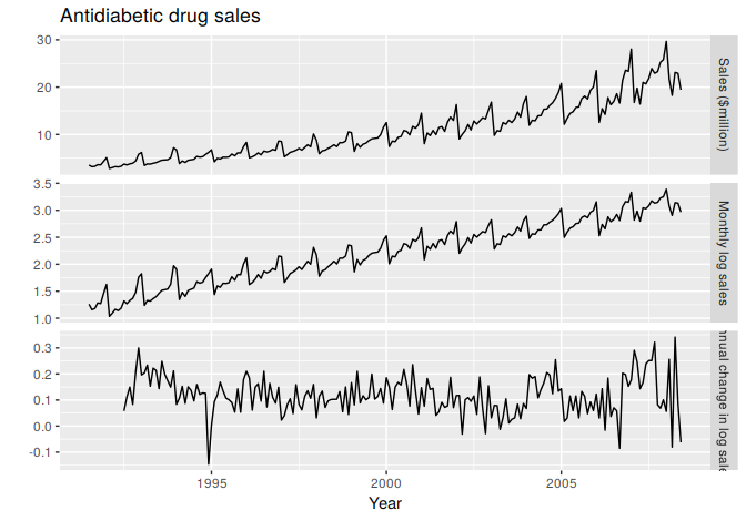

Figure 8.3: Logs and seasonal differences of the A10 (antidiabetic) sales data. The logarithms stabilize the variance, while the seasonal differences remove the seasonality and trend.

Figure 8.3 shows the seasonal differences of the logarithm of the monthly scripts for A10 (antidiabetic) drugs sold in Australia. The transformation and differencing have made the series look relatively stationary.

To distinguish seasonal differences from ordinary differences, we sometimes refer to ordinary differences as “first differences”, meaning differences at lag 1.

Sometimes it is necessary to do both a seasonal difference and a first difference to obtain stationary data, as is shown in Figure 8.4. Here, the data are first transformed using logarithms (second panel), then seasonal differences are calculated (third panel). The data still seem a little non-stationary, and so a further lot of first differences are computed (bottom panel).

cbind("Billion kWh" = usmelec,
      "Logs" = log(usmelec),
      "Seasonally\n differenced logs" = diff(log(usmelec),12),
      "Doubly\n differenced logs" = diff(diff(log(usmelec),12),1)) %>%
  autoplot(facets=TRUE) +
    xlab("Year") + ylab("") +
    ggtitle("Monthly US net electricity generation")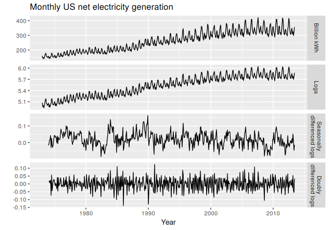

Figure 8.4: Top panel: US net electricity generation (billion kWh). Other panels show the same data after transforming and differencing.

There is a degree of subjectivity in selecting which differences to apply. The seasonally differenced data in Figure 8.3 do not show substantially different behaviour from the seasonally differenced data in Figure 8.4. In the latter case, we could have decided to stop with the seasonally differenced data, and not done an extra round of differencing. In the former case, we could have decided that the data were not sufficiently stationary and taken an extra round of differencing. Some formal tests for differencing will be discussed later, but there are always some choices to be made in the modeling process, and different analysts may make different choices.

If \(y'_t = y_t - y_{t-m}\) denotes a seasonally differenced series, then the twice-differenced series is \[\begin{align*} y''_t &= y'_t - y'_{t-1} \\ &= (y_t - y_{t-m}) - (y_{t-1} - y_{t-m-1}) \\ &= y_t -y_{t-1} - y_{t-m} + y_{t-m-1}\: \end{align*}\] When both seasonal and first differences are applied, it makes no difference which is done first—the result will be the same. However, if the data have a strong seasonal pattern, we recommend that seasonal differencing be done first, because the resulting series will sometimes be stationary and there will be no need for a further first difference. If first differencing is done first, there will still be seasonality present.

It is important that if differencing is used, the differences are interpretable. First differences are the change between one observation and the next. Seasonal differences are the change between one year to the next. Other lags are unlikely to make much interpretable sense and should be avoided.

Unit root tests

One way to determine more objectively whether differencing is required is to use a unit root test. These are statistical hypothesis tests of stationarity that are designed for determining whether differencing is required.

A number of different unit root tests are available, which are based on different assumptions and may lead to conflicting answers.

ADF test

One of the most popular tests is the Augmented Dickey-Fuller (ADF) test. For this test, the following regression model is estimated: \[ y'_t = \alpha + \beta t + \phi y_{t-1} + \gamma_1 y'_{t-1} + \gamma_2 y'_{t-2} + \cdots + \gamma_k y'_{t-k}, \] where \(y'_t\) denotes the first-differenced series, \(y'_t=y_t-y_{t-1}\), and \(k\) is the number of lags to include in the regression (often set to be about 3). If the original series, \(y_t\), needs differencing, then the coefficient \(\hat\phi\) should be approximately zero. If \(y_t\) is already stationary, then \(\hat{\phi}<0\). The usual hypothesis tests for regression coefficients do not work when the data are non-stationary, but the test can be carried out using the following R function from the tseries package.

adf.test(x, alternative = "stationary")

In R, the default value of \(k\) is set to \(\lfloor(T - 1)^{1/3}\rfloor\), where \(T\) is the length of the time series and \(\lfloor x\rfloor\) means the largest integer not greater than \(x\).

The null-hypothesis for an ADF test is that the data are non-stationary. Thus, large p-values are indicative of non-stationarity, and small p-values suggest stationarity. Using the usual 5% threshold, differencing is required if the p-value is greater than 0.05.

KPSS test

Another popular unit root test is the Kwiatkowski-Phillips-Schmidt-Shin (KPSS) test. This reverses the hypotheses, so the null hypothesis is that the data are stationary. In this case, small p-values (e.g., less than 0.05) suggest that differencing is required. The kpss.test is also from the tseries package.

kpss.test(x)

A useful R function is ndiffs(), which uses these tests to determine the appropriate number of first differences required for a non-seasonal time series.

More complicated tests are required for seasonal differencing, and are beyond the scope of this book. A useful R function for determining whether seasonal differencing is required is nsdiffs(), which uses seasonal unit root tests to determine the appropriate number of seasonal differences required.

The following code can be used to find how to make a seasonal series stationary. The resulting series, stored as xstar, has been differenced appropriately.

ns <- nsdiffs(x)
if(ns > 0)
  xstar <- diff(x, lag=frequency(x), differences=ns)
else
  xstar <- x
nd <- ndiffs(xstar)
if(nd > 0)
  xstar <- diff(xstar, differences=nd)

---

14. More precisely, if \(\{y_t\}\) is a stationary time series, then for all \(s\), the distribution of \((y_t,\dots,y_{t+s})\) does not depend on \(t\).↩