9.6 Lagged predictors

Sometimes, the impact of a predictor which is included in a regression model will not be simple and immediate. For example, an advertising campaign may impact sales for some time beyond the end of the campaign, and sales in one month will depend on the advertising expenditure in each of the past few months. Similarly, a change in a company’s safety policy may reduce accidents immediately, but have a diminishing effect over time as employees take less care when they become familiar with the new working conditions.

In these situations, we need to allow for lagged effects of the predictor. Suppose that we have only one predictor in our model. Then a model which allows for lagged effects can be written as \[ y_t = \beta_0 + \gamma_0x_t + \gamma_1 x_{t-1} + \dots + \gamma_k x_{t-k} + n_t, \] where \(n_t\) is an ARIMA process. The value of \(k\) can be selected using the AICc, along with the values of \(p\) and \(q\) for the ARIMA error.

Example: TV advertising and insurance quotations

A US insurance company advertises on national television in an attempt to increase the number of insurance quotations provided (and consequently the number of new policies). Figure 9.9 shows the number of quotations and the expenditure on television advertising for the company each month from January 2002 to April 2005.

autoplot(insurance, facets=TRUE) +
  xlab("Year") + ylab("") +
  ggtitle("Insurance advertising and quotations")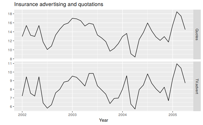

Figure 9.9: Numbers of insurance quotations provided per month and the expenditure on advertising per month.

We will consider including advertising expenditure for up to four months; that is, the model may include advertising expenditure in the current month, and the three months before that. When comparing models, it is important that they all use the same training set. In the following code, we exclude the first three months in order to make fair comparisons. The best model is the one with the smallest AICc value.

# Lagged predictors. Test 0, 1, 2 or 3 lags.
# Advert <- cbind(
#   AdLag0 = insurance[,"TV.advert"],
#   AdLag1 = lag(insurance[,"TV.advert"],-1),
#   AdLag2 = lag(insurance[,"TV.advert"],-2),
#   AdLag3 = lag(insurance[,"TV.advert"],-3))[1:NROW(insurance),]

# Choose optimal lag length for advertising based on AICc
# Restrict data so models use same fitting period
# fit1 <- auto.arima(insurance[4:40,1], xreg=Advert[4:40,1], d=0)
# fit2 <- auto.arima(insurance[4:40,1], xreg=Advert[4:40,1:2], d=0)
# fit3 <- auto.arima(insurance[4:40,1], xreg=Advert[4:40,1:3], d=0)
# fit4 <- auto.arima(insurance[4:40,1], xreg=Advert[4:40,1:4], d=0)

# Best model fitted to all data (based on AICc)
# Refit using all data
# (fit <- auto.arima(insurance[,1], xreg=Advert[,1:2], d=0))

The chosen model includes advertising only in the current month and the previous month, and has AR(3) errors. The model can be written as \[ y_t = NA + NA x_t + NA x_{t-1} + n_t, \] where \(y_t\) is the number of quotations provided in month \(t\), \(x_t\) is the advertising expenditure in month \(t\), \[ n_t = NA n_{t-1} NA n_{t-2} + NA n_{t-3} + e_t, \] and \(e_t\) is white noise.

We can calculate forecasts using this model if we assume future values for the advertising variable. If we set the future monthly advertising to 8 units, we get the following forecasts.

# fc8 <- forecast(fit, h=20,
#   xreg=cbind(AdLag0=rep(8,20), AdLag1=c(Advert[40,1],rep(8,19))))
# autoplot(fc8) + ylab("Quotes") +
#   ggtitle("Forecast quotes with future advertising set to 8")