12.2 Time series of counts
All of the methods discussed in this book assume that the data have a continuous sample space. But very often data comes in the form of counts. For example, we may wish to forecast the number of customers who enter a store each day. We could have 0, 1, 2, , customers, but we cannot have 3.45693 customers.
In practice, this rarely matters provided our counts are sufficiently large. If the minimum number of customers is at least 100, then the difference between a continuous sample space \([100,\infty)\) and the discrete sample space \(\{100,101,102,\dots\}\) has no perceivable effect on our forecasts. However, if our data contains small counts \((0, 1, 2, \dots)\), then we need to use forecasting methods that are more appropriate for a sample space of non-negative integers.
Such models are beyond the scope of this book. However, there is one simple method which gets used in this context, that we would like to mention. It is “Croston’s method”, named after its British inventor, John Croston, and first described in Croston (1972). Actually, this method does not properly deal with the count nature of the data either, but it is used so often, that it is worth knowing about it.
With Croston’s method, we construct two new series from our original time series by noting which time periods contain zero values, and which periods contain non-zero values. Let \(q_i\) be the \(i\)th non-zero quantity, and let \(a_i\) be the time between \(q_{i-1}\) and \(q_i\). Croston’s method involves separate simple exponential smoothing forecasts on the two new series \(a\) and \(q\). Because the method is usually applied to time series of demand for items, \(q\) is often called the “demand” and \(a\) the “inter-arrival time”.
If \(\hat{q}_{i+1|i}\) and \(\hat{a}_{i+1|i}\) are the one-step forecasts of the \((i+1)\)th demand and inter-arrival time respectively, based on data up to demand \(i\), then Croston’s method gives \[\begin{align} \hat{q}_{i+1|i} & = (1-\alpha)\hat{q}_{i|i-1} + \alpha q_i, \tag{12.1}\\ \hat{a}_{i+1|i} & = (1-\alpha)\hat{a}_{i|i-1} + \alpha a_i. \tag{12.2} \end{align}\] The smoothing parameter \(\alpha\) takes values between 0 and 1 and is assumed to be the same for both equations. Let \(j\) be the time for the last observed positive observation. Then the \(h\)-step ahead forecast for the demand at time \(T+h\), is given by the ratio \[\begin{equation}\label{c2ratio} \hat{y}_{T+h|T} = q_{j+1|j}/a_{j+1|j}. \end{equation}\]
There are no algebraic results allowing us to compute prediction intervals for this method, because the method does not correspond to any statistical model (Shenstone and Hyndman 2005).
The croston function produces forecasts using Croston’s method. In the following example, we apply the method to monthly sales of a lubricant that is rarely used. This data set was part of a consulting project that one of us did for an oil company several years ago.
The data contain small counts, with many months registering no sales at all, and only small numbers of items sold in other months.
| Jan | Feb | Mar | Apr | May | Jun | Jul | Aug | Sep | Oct | Nov | Dec |
|---|---|---|---|---|---|---|---|---|---|---|---|
| 0 | 2 | 0 | 1 | 0 | 11 | 0 | 0 | 0 | 0 | 2 | 0 |
| 6 | 3 | 0 | 0 | 0 | 0 | 0 | 7 | 0 | 0 | 0 | 0 |
| 0 | 0 | 0 | 3 | 1 | 0 | 0 | 1 | 0 | 1 | 0 | 0 |
The demand and arrival series are computed from the above data.
| i | q | a |
|---|---|---|
| 1 | 2 | 2 |
| 2 | 1 | 2 |
| 3 | 11 | 2 |
| 4 | 2 | 5 |
| 5 | 6 | 2 |
| 6 | 3 | 1 |
| 7 | 7 | 6 |
| 8 | 3 | 8 |
| 9 | 1 | 1 |
| 10 | 1 | 3 |
| 11 | 1 | 2 |
The croston function simply uses \(\alpha=0.1\) by default, and \(\ell_0\) is set to be equal to the first observation in each of the series. This is consistent with the way Croston envisaged the method being used. This gives the demand forecast 2.750 and the arrival forecast 2.793. So the forecast of the original series is
\(\hat{y}_{T+h|T} = 2.750 / 2.793 = 0.985\). In practice, R does these calculations for you:
productC %>% croston() %>% autoplot()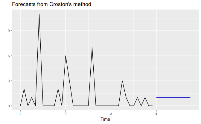
An implementation of Croston’s method with more facilities (including parameter estimation) is available in the tsintermittent package for R.
Forecasting models that deal more directly with the count nature of the data are described in Christou and Fokianos (2015).
References
Christou, Vasiliki, and Konstantinos Fokianos. 2015. “On Count Time Series Prediction.” Journal of Statistical Computation and Simulation 85 (2): 357–73.
Croston, John D. 1972. “Forecasting and Stock Control for Intermittent Demands.” Operational Research Quarterly 23 (3): 289–303.
Shenstone, Lydia, and Rob J Hyndman. 2005. “Stochastic Models Underlying Croston’s Method for Intermittent Demand Forecasting.” Journal of Forecasting 24 (6): 389–402. dx.doi.org/10.1002/for.963.