3.5 Prediction intervals
As discussed in Section 1.7, a prediction interval gives an interval within which we expect \(y_{t}\) to lie with a specified probability. For example, assuming that the forecast errors are normally distributed, a 95% prediction interval for the \(h\)-step forecast is \[ \hat{y}_{T+h|T} \pm 1.96 \hat\sigma_h, \] where \(\hat\sigma_h\) is an estimate of the standard deviation of the \(h\)-step forecast distribution.
More generally, a prediction interval can be written as \[ \hat{y}_{T+h|T} \pm k \hat\sigma_h \] where the multiplier \(k\) depends on the coverage probability. In this book we usually calculate 80% intervals and 95% intervals, although any percentage may be used. The following table gives the value of \(k\) for a range of coverage probabilities assuming normally distributed forecast errors.
| Percentage | Multiplier |
|---|---|
| 50 | 0.67 |
| 55 | 0.76 |
| 60 | 0.84 |
| 65 | 0.93 |
| 70 | 1.04 |
| 75 | 1.15 |
| 80 | 1.28 |
| 85 | 1.44 |
| 90 | 1.64 |
| 95 | 1.96 |
| 96 | 2.05 |
| 97 | 2.17 |
| 98 | 2.33 |
| 99 | 2.58 |
The value of prediction intervals is that they express the uncertainty in the forecasts. If we only produce point forecasts, there is no way of telling how accurate the forecasts are. However, if we also produce prediction intervals, then it is clear how much uncertainty is associated with each forecast. For this reason, point forecasts can be of almost no value without the accompanying prediction intervals.
One-step prediction intervals
When forecasting one step ahead, the standard deviation of the forecast distribution is almost the same as the standard deviation of the residuals. (In fact, the two standard deviations are identical if there are no parameters to be estimated, as is the case with the naïve method. For forecasting methods involving parameters to be estimated, the standard deviation of the forecast distribution is slightly larger than the residual standard deviation, although this difference is often ignored.)
For example, consider a naïve forecast for the Dow-Jones Index. The last value of the observed series is 3830, so the forecast of the next value of the DJI is 3830. The standard deviation of the residuals from the naïve method is 22.00 . Hence, a 95% prediction interval for the next value of the DJI is \[ 3830 \pm 1.96(22.00) = [3787, 3873]. \] Similarly, an 80% prediction interval is given by \[ 3830 \pm 1.28(22.00) = [3802, 3858]. \]
The value of the multiplier (1.96 or 1.28) is taken from Table 3.1.
Multi-step prediction intervals
A common feature of prediction intervals is that they increase in length as the forecast horizon increases. The further ahead we forecast, the more uncertainty is associated with the forecast, and thus the wider the prediction intervals. That is, \(\sigma_h\) usually increases with \(h\) (although there are some non-linear forecasting methods that do not have this property).
To produce a prediction interval, it is necessary to have an estimate of \(\sigma_h\). As already noted, for one-step forecasts (\(h=1\)), the residual standard deviation provides a good estimate of the forecast standard deviation \(\sigma_1\). For multi-step forecasts, a more complicated method of calculation is required. These calculations assume that the residuals are uncorrelated.
Benchmark methods
For the four benchmark methods, it is possible to mathematically derive the forecast standard deviation under the assumption of uncorrelated residuals. If \(\hat{\sigma}_h\) denotes the standard deviation of the \(h\)-step forecast distribution, and \(\hat{\sigma}\) is the residual standard deviation, then we can use the following expressions.
Mean forecasts: \(\hat\sigma_h = \hat\sigma\sqrt{1 + 1/T}\)
Naïve forecasts: \(\hat\sigma_h = \hat\sigma\sqrt{h}\)
Seasonal naïve forecasts \(\hat\sigma_h = \hat\sigma\sqrt{\lfloor (h-1)/m \rfloor + 1}\).
Drift forecasts: \(\hat\sigma_h = \hat\sigma\sqrt{h(1+h/T)}\).
Note that when \(h=1\) and \(T\) is large, these all give the same approximate value \(\hat\sigma\).
Prediction intervals will be computed for you when using any of the benchmark forecasting methods. For example, here is the output when using the naïve method for the Dow-Jones index.
naive(dj2)
#>     Point Forecast Lo 80 Hi 80 Lo 95 Hi 95
#> 251           3830  3802  3858  3787  3873
#> 252           3830  3790  3870  3769  3891
#> 253           3830  3781  3879  3755  3905
#> 254           3830  3774  3886  3744  3916
#> 255           3830  3767  3893  3734  3926
#> 256           3830  3761  3899  3724  3936
#> 257           3830  3755  3905  3716  3944
#> 258           3830  3750  3910  3708  3952
#> 259           3830  3745  3915  3701  3959
#> 260           3830  3741  3919  3694  3966
When plotted, the prediction intervals are shown as shaded region, with the strength of colour indicating the probability associated with the interval.
autoplot(naive(dj2))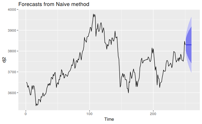
Bootstrapped prediction intervals
When a normal distribution for the forecast errors is an unreasonable assumption, one alternative is to use bootstrapping, which only assumes that the forecast errors are uncorrelated.
A forecast error is defined as \(e_t = y_t - \hat{y}_{t|t-1}\). We can re-write this as \[ y_t = \hat{y}_{t|t-1} + e_t. \] So we can simulate the next observation of a time series using \[ y_{T+1} = \hat{y}_{T+1|T} + e_{T+1} \] where \(\hat{y}_{T+1|T}\) is the one-step forecast and \(e_{T+1}\) is the unknown future error. Assuming future errors will be similar to past errors, we can replace \(e_{T+1}\) by sampling from the collection of errors we have seen in the past (i.e., the residuals). Adding the new simulated observation to our data set, we can repeat the process to obtain \[ y_{T+2} = \hat{y}_{T+2|T+1} + e_{T+2} \] where \(e_{T+2}\) is another draw from the collection of residuals. Continuing in this way, we can simulate an entire set of future values for our time series.
Doing this repeatedly, we obtain many possible futures. Then we can compute prediction intervals by calculating percentiles for each forecast horizon. The result is called a “bootstrapped” prediction interval. The name “bootstrap” is a reference to pulling ourselves up by our bootstraps, because the process allows us to measure future uncertainty by only using the historical data.
To generate such intervals, we can simply add the bootstrap argument to our forecasting functions. For example:
naive(dj2, bootstrap=TRUE)
#>     Point Forecast Lo 80 Hi 80 Lo 95 Hi 95
#> 251           3830  3803  3854  3781  3871
#> 252           3830  3790  3868  3763  3889
#> 253           3830  3782  3877  3750  3900
#> 254           3830  3775  3883  3735  3913
#> 255           3830  3768  3888  3727  3922
#> 256           3830  3761  3895  3718  3933
#> 257           3830  3753  3901  3708  3941
#> 258           3830  3749  3906  3698  3946
#> 259           3830  3746  3912  3690  3957
#> 260           3830  3740  3917  3687  3961
In this case, they are very similar (but not identical) to the prediction intervals based on the normal distribution.
Prediction intervals with transformations
If a transformation has been used, then the prediction interval should be computed on the transformed scale, and the end points back-transformed to give a prediction interval on the original scale. This approach preserves the probability coverage of the prediction interval, although it will no longer be symmetric around the point forecast.
The back-transformation of prediction intervals is done automatically using the functions in the forecast package in R, provided you have used the lambda argument when computing the forecasts.