40 Wine classification with neuralnet
Source: https://www.r-bloggers.com/multilabel-classification-with-neuralnet-package/
The neuralnet package is perhaps not the best option in R for using neural networks. If you ask why, for starters it does not recognize the typical formula y~., it does not support factors, it does not provide a lot of models other than a standard MLP, and it has great competitors in the nnet package that seems to be better integrated in R and can be used with the caret package, and in the MXnet package that is a high level deep learning library which provides a wide variety of neural networks.
But still, I think there is some value in the ease of use of the neuralnet package, especially for a beginner, therefore I’ll be using it.
I’m going to be using both the neuralnet and, curiously enough, the nnet package. Let’s load them:
# load libs
require(neuralnet)
#> Loading required package: neuralnet
require(nnet)
#> Loading required package: nnet
require(ggplot2)
#> Loading required package: ggplot2
set.seed(10)
40.1 The dataset
I looked in the UCI Machine Learning Repository1 and found the wine dataset.
This dataset contains the results of a chemical analysis on 3 different kind of wines. The target variable is the label of the wine which is a factor with 3 (unordered) levels. The predictors are all continuous and represent 13 variables obtained as a result of chemical measurements.
# get the data file from the package location
wine_dataset_path <- file.path(data_raw_dir, "wine.data")
wine_dataset_path
#> [1] "../data/wine.data"
wines <- read.csv(wine_dataset_path)
wines
#>     X1 X14.23 X1.71 X2.43 X15.6 X127 X2.8 X3.06 X.28 X2.29 X5.64 X1.04 X3.92
#> 1    1   13.2  1.78  2.14  11.2  100 2.65  2.76 0.26  1.28  4.38 1.050  3.40
#> 2    1   13.2  2.36  2.67  18.6  101 2.80  3.24 0.30  2.81  5.68 1.030  3.17
#> 3    1   14.4  1.95  2.50  16.8  113 3.85  3.49 0.24  2.18  7.80 0.860  3.45
#> 4    1   13.2  2.59  2.87  21.0  118 2.80  2.69 0.39  1.82  4.32 1.040  2.93
#> 5    1   14.2  1.76  2.45  15.2  112 3.27  3.39 0.34  1.97  6.75 1.050  2.85
#> 6    1   14.4  1.87  2.45  14.6   96 2.50  2.52 0.30  1.98  5.25 1.020  3.58
#> 7    1   14.1  2.15  2.61  17.6  121 2.60  2.51 0.31  1.25  5.05 1.060  3.58
#> 8    1   14.8  1.64  2.17  14.0   97 2.80  2.98 0.29  1.98  5.20 1.080  2.85
#> 9    1   13.9  1.35  2.27  16.0   98 2.98  3.15 0.22  1.85  7.22 1.010  3.55
#> 10   1   14.1  2.16  2.30  18.0  105 2.95  3.32 0.22  2.38  5.75 1.250  3.17
#> 11   1   14.1  1.48  2.32  16.8   95 2.20  2.43 0.26  1.57  5.00 1.170  2.82
#> 12   1   13.8  1.73  2.41  16.0   89 2.60  2.76 0.29  1.81  5.60 1.150  2.90
#> 13   1   14.8  1.73  2.39  11.4   91 3.10  3.69 0.43  2.81  5.40 1.250  2.73
#> 14   1   14.4  1.87  2.38  12.0  102 3.30  3.64 0.29  2.96  7.50 1.200  3.00
#> 15   1   13.6  1.81  2.70  17.2  112 2.85  2.91 0.30  1.46  7.30 1.280  2.88
#> 16   1   14.3  1.92  2.72  20.0  120 2.80  3.14 0.33  1.97  6.20 1.070  2.65
#> 17   1   13.8  1.57  2.62  20.0  115 2.95  3.40 0.40  1.72  6.60 1.130  2.57
#> 18   1   14.2  1.59  2.48  16.5  108 3.30  3.93 0.32  1.86  8.70 1.230  2.82
#> 19   1   13.6  3.10  2.56  15.2  116 2.70  3.03 0.17  1.66  5.10 0.960  3.36
#> 20   1   14.1  1.63  2.28  16.0  126 3.00  3.17 0.24  2.10  5.65 1.090  3.71
#> 21   1   12.9  3.80  2.65  18.6  102 2.41  2.41 0.25  1.98  4.50 1.030  3.52
#> 22   1   13.7  1.86  2.36  16.6  101 2.61  2.88 0.27  1.69  3.80 1.110  4.00
#> 23   1   12.8  1.60  2.52  17.8   95 2.48  2.37 0.26  1.46  3.93 1.090  3.63
#> 24   1   13.5  1.81  2.61  20.0   96 2.53  2.61 0.28  1.66  3.52 1.120  3.82
#> 25   1   13.1  2.05  3.22  25.0  124 2.63  2.68 0.47  1.92  3.58 1.130  3.20
#> 26   1   13.4  1.77  2.62  16.1   93 2.85  2.94 0.34  1.45  4.80 0.920  3.22
#> 27   1   13.3  1.72  2.14  17.0   94 2.40  2.19 0.27  1.35  3.95 1.020  2.77
#> 28   1   13.9  1.90  2.80  19.4  107 2.95  2.97 0.37  1.76  4.50 1.250  3.40
#> 29   1   14.0  1.68  2.21  16.0   96 2.65  2.33 0.26  1.98  4.70 1.040  3.59
#> 30   1   13.7  1.50  2.70  22.5  101 3.00  3.25 0.29  2.38  5.70 1.190  2.71
#> 31   1   13.6  1.66  2.36  19.1  106 2.86  3.19 0.22  1.95  6.90 1.090  2.88
#> 32   1   13.7  1.83  2.36  17.2  104 2.42  2.69 0.42  1.97  3.84 1.230  2.87
#> 33   1   13.8  1.53  2.70  19.5  132 2.95  2.74 0.50  1.35  5.40 1.250  3.00
#> 34   1   13.5  1.80  2.65  19.0  110 2.35  2.53 0.29  1.54  4.20 1.100  2.87
#> 35   1   13.5  1.81  2.41  20.5  100 2.70  2.98 0.26  1.86  5.10 1.040  3.47
#> 36   1   13.3  1.64  2.84  15.5  110 2.60  2.68 0.34  1.36  4.60 1.090  2.78
#> 37   1   13.1  1.65  2.55  18.0   98 2.45  2.43 0.29  1.44  4.25 1.120  2.51
#> 38   1   13.1  1.50  2.10  15.5   98 2.40  2.64 0.28  1.37  3.70 1.180  2.69
#> 39   1   14.2  3.99  2.51  13.2  128 3.00  3.04 0.20  2.08  5.10 0.890  3.53
#> 40   1   13.6  1.71  2.31  16.2  117 3.15  3.29 0.34  2.34  6.13 0.950  3.38
#> 41   1   13.4  3.84  2.12  18.8   90 2.45  2.68 0.27  1.48  4.28 0.910  3.00
#> 42   1   13.9  1.89  2.59  15.0  101 3.25  3.56 0.17  1.70  5.43 0.880  3.56
#> 43   1   13.2  3.98  2.29  17.5  103 2.64  2.63 0.32  1.66  4.36 0.820  3.00
#> 44   1   13.1  1.77  2.10  17.0  107 3.00  3.00 0.28  2.03  5.04 0.880  3.35
#> 45   1   14.2  4.04  2.44  18.9  111 2.85  2.65 0.30  1.25  5.24 0.870  3.33
#> 46   1   14.4  3.59  2.28  16.0  102 3.25  3.17 0.27  2.19  4.90 1.040  3.44
#> 47   1   13.9  1.68  2.12  16.0  101 3.10  3.39 0.21  2.14  6.10 0.910  3.33
#> 48   1   14.1  2.02  2.40  18.8  103 2.75  2.92 0.32  2.38  6.20 1.070  2.75
#> 49   1   13.9  1.73  2.27  17.4  108 2.88  3.54 0.32  2.08  8.90 1.120  3.10
#> 50   1   13.1  1.73  2.04  12.4   92 2.72  3.27 0.17  2.91  7.20 1.120  2.91
#> 51   1   13.8  1.65  2.60  17.2   94 2.45  2.99 0.22  2.29  5.60 1.240  3.37
#> 52   1   13.8  1.75  2.42  14.0  111 3.88  3.74 0.32  1.87  7.05 1.010  3.26
#> 53   1   13.8  1.90  2.68  17.1  115 3.00  2.79 0.39  1.68  6.30 1.130  2.93
#> 54   1   13.7  1.67  2.25  16.4  118 2.60  2.90 0.21  1.62  5.85 0.920  3.20
#> 55   1   13.6  1.73  2.46  20.5  116 2.96  2.78 0.20  2.45  6.25 0.980  3.03
#> 56   1   14.2  1.70  2.30  16.3  118 3.20  3.00 0.26  2.03  6.38 0.940  3.31
#> 57   1   13.3  1.97  2.68  16.8  102 3.00  3.23 0.31  1.66  6.00 1.070  2.84
#> 58   1   13.7  1.43  2.50  16.7  108 3.40  3.67 0.19  2.04  6.80 0.890  2.87
#> 59   2   12.4  0.94  1.36  10.6   88 1.98  0.57 0.28  0.42  1.95 1.050  1.82
#> 60   2   12.3  1.10  2.28  16.0  101 2.05  1.09 0.63  0.41  3.27 1.250  1.67
#> 61   2   12.6  1.36  2.02  16.8  100 2.02  1.41 0.53  0.62  5.75 0.980  1.59
#> 62   2   13.7  1.25  1.92  18.0   94 2.10  1.79 0.32  0.73  3.80 1.230  2.46
#> 63   2   12.4  1.13  2.16  19.0   87 3.50  3.10 0.19  1.87  4.45 1.220  2.87
#> 64   2   12.2  1.45  2.53  19.0  104 1.89  1.75 0.45  1.03  2.95 1.450  2.23
#> 65   2   12.4  1.21  2.56  18.1   98 2.42  2.65 0.37  2.08  4.60 1.190  2.30
#> 66   2   13.1  1.01  1.70  15.0   78 2.98  3.18 0.26  2.28  5.30 1.120  3.18
#> 67   2   12.4  1.17  1.92  19.6   78 2.11  2.00 0.27  1.04  4.68 1.120  3.48
#> 68   2   13.3  0.94  2.36  17.0  110 2.53  1.30 0.55  0.42  3.17 1.020  1.93
#> 69   2   12.2  1.19  1.75  16.8  151 1.85  1.28 0.14  2.50  2.85 1.280  3.07
#> 70   2   12.3  1.61  2.21  20.4  103 1.10  1.02 0.37  1.46  3.05 0.906  1.82
#> 71   2   13.9  1.51  2.67  25.0   86 2.95  2.86 0.21  1.87  3.38 1.360  3.16
#> 72   2   13.5  1.66  2.24  24.0   87 1.88  1.84 0.27  1.03  3.74 0.980  2.78
#> 73   2   13.0  1.67  2.60  30.0  139 3.30  2.89 0.21  1.96  3.35 1.310  3.50
#> 74   2   12.0  1.09  2.30  21.0  101 3.38  2.14 0.13  1.65  3.21 0.990  3.13
#> 75   2   11.7  1.88  1.92  16.0   97 1.61  1.57 0.34  1.15  3.80 1.230  2.14
#> 76   2   13.0  0.90  1.71  16.0   86 1.95  2.03 0.24  1.46  4.60 1.190  2.48
#> 77   2   11.8  2.89  2.23  18.0  112 1.72  1.32 0.43  0.95  2.65 0.960  2.52
#> 78   2   12.3  0.99  1.95  14.8  136 1.90  1.85 0.35  2.76  3.40 1.060  2.31
#> 79   2   12.7  3.87  2.40  23.0  101 2.83  2.55 0.43  1.95  2.57 1.190  3.13
#> 80   2   12.0  0.92  2.00  19.0   86 2.42  2.26 0.30  1.43  2.50 1.380  3.12
#> 81   2   12.7  1.81  2.20  18.8   86 2.20  2.53 0.26  1.77  3.90 1.160  3.14
#> 82   2   12.1  1.13  2.51  24.0   78 2.00  1.58 0.40  1.40  2.20 1.310  2.72
#> 83   2   13.1  3.86  2.32  22.5   85 1.65  1.59 0.61  1.62  4.80 0.840  2.01
#> 84   2   11.8  0.89  2.58  18.0   94 2.20  2.21 0.22  2.35  3.05 0.790  3.08
#> 85   2   12.7  0.98  2.24  18.0   99 2.20  1.94 0.30  1.46  2.62 1.230  3.16
#> 86   2   12.2  1.61  2.31  22.8   90 1.78  1.69 0.43  1.56  2.45 1.330  2.26
#> 87   2   11.7  1.67  2.62  26.0   88 1.92  1.61 0.40  1.34  2.60 1.360  3.21
#> 88   2   11.6  2.06  2.46  21.6   84 1.95  1.69 0.48  1.35  2.80 1.000  2.75
#> 89   2   12.1  1.33  2.30  23.6   70 2.20  1.59 0.42  1.38  1.74 1.070  3.21
#> 90   2   12.1  1.83  2.32  18.5   81 1.60  1.50 0.52  1.64  2.40 1.080  2.27
#> 91   2   12.0  1.51  2.42  22.0   86 1.45  1.25 0.50  1.63  3.60 1.050  2.65
#> 92   2   12.7  1.53  2.26  20.7   80 1.38  1.46 0.58  1.62  3.05 0.960  2.06
#> 93   2   12.3  2.83  2.22  18.0   88 2.45  2.25 0.25  1.99  2.15 1.150  3.30
#> 94   2   11.6  1.99  2.28  18.0   98 3.02  2.26 0.17  1.35  3.25 1.160  2.96
#> 95   2   12.5  1.52  2.20  19.0  162 2.50  2.27 0.32  3.28  2.60 1.160  2.63
#> 96   2   11.8  2.12  2.74  21.5  134 1.60  0.99 0.14  1.56  2.50 0.950  2.26
#> 97   2   12.3  1.41  1.98  16.0   85 2.55  2.50 0.29  1.77  2.90 1.230  2.74
#> 98   2   12.4  1.07  2.10  18.5   88 3.52  3.75 0.24  1.95  4.50 1.040  2.77
#> 99   2   12.3  3.17  2.21  18.0   88 2.85  2.99 0.45  2.81  2.30 1.420  2.83
#> 100  2   12.1  2.08  1.70  17.5   97 2.23  2.17 0.26  1.40  3.30 1.270  2.96
#> 101  2   12.6  1.34  1.90  18.5   88 1.45  1.36 0.29  1.35  2.45 1.040  2.77
#> 102  2   12.3  2.45  2.46  21.0   98 2.56  2.11 0.34  1.31  2.80 0.800  3.38
#> 103  2   11.8  1.72  1.88  19.5   86 2.50  1.64 0.37  1.42  2.06 0.940  2.44
#> 104  2   12.5  1.73  1.98  20.5   85 2.20  1.92 0.32  1.48  2.94 1.040  3.57
#> 105  2   12.4  2.55  2.27  22.0   90 1.68  1.84 0.66  1.42  2.70 0.860  3.30
#> 106  2   12.2  1.73  2.12  19.0   80 1.65  2.03 0.37  1.63  3.40 1.000  3.17
#> 107  2   12.7  1.75  2.28  22.5   84 1.38  1.76 0.48  1.63  3.30 0.880  2.42
#> 108  2   12.2  1.29  1.94  19.0   92 2.36  2.04 0.39  2.08  2.70 0.860  3.02
#> 109  2   11.6  1.35  2.70  20.0   94 2.74  2.92 0.29  2.49  2.65 0.960  3.26
#> 110  2   11.5  3.74  1.82  19.5  107 3.18  2.58 0.24  3.58  2.90 0.750  2.81
#> 111  2   12.5  2.43  2.17  21.0   88 2.55  2.27 0.26  1.22  2.00 0.900  2.78
#> 112  2   11.8  2.68  2.92  20.0  103 1.75  2.03 0.60  1.05  3.80 1.230  2.50
#> 113  2   11.4  0.74  2.50  21.0   88 2.48  2.01 0.42  1.44  3.08 1.100  2.31
#> 114  2   12.1  1.39  2.50  22.5   84 2.56  2.29 0.43  1.04  2.90 0.930  3.19
#> 115  2   11.0  1.51  2.20  21.5   85 2.46  2.17 0.52  2.01  1.90 1.710  2.87
#> 116  2   11.8  1.47  1.99  20.8   86 1.98  1.60 0.30  1.53  1.95 0.950  3.33
#> 117  2   12.4  1.61  2.19  22.5  108 2.00  2.09 0.34  1.61  2.06 1.060  2.96
#> 118  2   12.8  3.43  1.98  16.0   80 1.63  1.25 0.43  0.83  3.40 0.700  2.12
#> 119  2   12.0  3.43  2.00  19.0   87 2.00  1.64 0.37  1.87  1.28 0.930  3.05
#> 120  2   11.4  2.40  2.42  20.0   96 2.90  2.79 0.32  1.83  3.25 0.800  3.39
#> 121  2   11.6  2.05  3.23  28.5  119 3.18  5.08 0.47  1.87  6.00 0.930  3.69
#> 122  2   12.4  4.43  2.73  26.5  102 2.20  2.13 0.43  1.71  2.08 0.920  3.12
#> 123  2   13.1  5.80  2.13  21.5   86 2.62  2.65 0.30  2.01  2.60 0.730  3.10
#> 124  2   11.9  4.31  2.39  21.0   82 2.86  3.03 0.21  2.91  2.80 0.750  3.64
#> 125  2   12.1  2.16  2.17  21.0   85 2.60  2.65 0.37  1.35  2.76 0.860  3.28
#> 126  2   12.4  1.53  2.29  21.5   86 2.74  3.15 0.39  1.77  3.94 0.690  2.84
#> 127  2   11.8  2.13  2.78  28.5   92 2.13  2.24 0.58  1.76  3.00 0.970  2.44
#> 128  2   12.4  1.63  2.30  24.5   88 2.22  2.45 0.40  1.90  2.12 0.890  2.78
#> 129  2   12.0  4.30  2.38  22.0   80 2.10  1.75 0.42  1.35  2.60 0.790  2.57
#> 130  3   12.9  1.35  2.32  18.0  122 1.51  1.25 0.21  0.94  4.10 0.760  1.29
#> 131  3   12.9  2.99  2.40  20.0  104 1.30  1.22 0.24  0.83  5.40 0.740  1.42
#> 132  3   12.8  2.31  2.40  24.0   98 1.15  1.09 0.27  0.83  5.70 0.660  1.36
#> 133  3   12.7  3.55  2.36  21.5  106 1.70  1.20 0.17  0.84  5.00 0.780  1.29
#> 134  3   12.5  1.24  2.25  17.5   85 2.00  0.58 0.60  1.25  5.45 0.750  1.51
#> 135  3   12.6  2.46  2.20  18.5   94 1.62  0.66 0.63  0.94  7.10 0.730  1.58
#> 136  3   12.2  4.72  2.54  21.0   89 1.38  0.47 0.53  0.80  3.85 0.750  1.27
#> 137  3   12.5  5.51  2.64  25.0   96 1.79  0.60 0.63  1.10  5.00 0.820  1.69
#> 138  3   13.5  3.59  2.19  19.5   88 1.62  0.48 0.58  0.88  5.70 0.810  1.82
#> 139  3   12.8  2.96  2.61  24.0  101 2.32  0.60 0.53  0.81  4.92 0.890  2.15
#> 140  3   12.9  2.81  2.70  21.0   96 1.54  0.50 0.53  0.75  4.60 0.770  2.31
#> 141  3   13.4  2.56  2.35  20.0   89 1.40  0.50 0.37  0.64  5.60 0.700  2.47
#> 142  3   13.5  3.17  2.72  23.5   97 1.55  0.52 0.50  0.55  4.35 0.890  2.06
#> 143  3   13.6  4.95  2.35  20.0   92 2.00  0.80 0.47  1.02  4.40 0.910  2.05
#> 144  3   12.2  3.88  2.20  18.5  112 1.38  0.78 0.29  1.14  8.21 0.650  2.00
#> 145  3   13.2  3.57  2.15  21.0  102 1.50  0.55 0.43  1.30  4.00 0.600  1.68
#> 146  3   13.9  5.04  2.23  20.0   80 0.98  0.34 0.40  0.68  4.90 0.580  1.33
#> 147  3   12.9  4.61  2.48  21.5   86 1.70  0.65 0.47  0.86  7.65 0.540  1.86
#> 148  3   13.3  3.24  2.38  21.5   92 1.93  0.76 0.45  1.25  8.42 0.550  1.62
#> 149  3   13.1  3.90  2.36  21.5  113 1.41  1.39 0.34  1.14  9.40 0.570  1.33
#> 150  3   13.5  3.12  2.62  24.0  123 1.40  1.57 0.22  1.25  8.60 0.590  1.30
#> 151  3   12.8  2.67  2.48  22.0  112 1.48  1.36 0.24  1.26 10.80 0.480  1.47
#> 152  3   13.1  1.90  2.75  25.5  116 2.20  1.28 0.26  1.56  7.10 0.610  1.33
#> 153  3   13.2  3.30  2.28  18.5   98 1.80  0.83 0.61  1.87 10.52 0.560  1.51
#> 154  3   12.6  1.29  2.10  20.0  103 1.48  0.58 0.53  1.40  7.60 0.580  1.55
#> 155  3   13.2  5.19  2.32  22.0   93 1.74  0.63 0.61  1.55  7.90 0.600  1.48
#> 156  3   13.8  4.12  2.38  19.5   89 1.80  0.83 0.48  1.56  9.01 0.570  1.64
#> 157  3   12.4  3.03  2.64  27.0   97 1.90  0.58 0.63  1.14  7.50 0.670  1.73
#> 158  3   14.3  1.68  2.70  25.0   98 2.80  1.31 0.53  2.70 13.00 0.570  1.96
#> 159  3   13.5  1.67  2.64  22.5   89 2.60  1.10 0.52  2.29 11.75 0.570  1.78
#> 160  3   12.4  3.83  2.38  21.0   88 2.30  0.92 0.50  1.04  7.65 0.560  1.58
#> 161  3   13.7  3.26  2.54  20.0  107 1.83  0.56 0.50  0.80  5.88 0.960  1.82
#> 162  3   12.8  3.27  2.58  22.0  106 1.65  0.60 0.60  0.96  5.58 0.870  2.11
#> 163  3   13.0  3.45  2.35  18.5  106 1.39  0.70 0.40  0.94  5.28 0.680  1.75
#> 164  3   13.8  2.76  2.30  22.0   90 1.35  0.68 0.41  1.03  9.58 0.700  1.68
#> 165  3   13.7  4.36  2.26  22.5   88 1.28  0.47 0.52  1.15  6.62 0.780  1.75
#> 166  3   13.4  3.70  2.60  23.0  111 1.70  0.92 0.43  1.46 10.68 0.850  1.56
#> 167  3   12.8  3.37  2.30  19.5   88 1.48  0.66 0.40  0.97 10.26 0.720  1.75
#> 168  3   13.6  2.58  2.69  24.5  105 1.55  0.84 0.39  1.54  8.66 0.740  1.80
#> 169  3   13.4  4.60  2.86  25.0  112 1.98  0.96 0.27  1.11  8.50 0.670  1.92
#> 170  3   12.2  3.03  2.32  19.0   96 1.25  0.49 0.40  0.73  5.50 0.660  1.83
#> 171  3   12.8  2.39  2.28  19.5   86 1.39  0.51 0.48  0.64  9.90 0.570  1.63
#> 172  3   14.2  2.51  2.48  20.0   91 1.68  0.70 0.44  1.24  9.70 0.620  1.71
#> 173  3   13.7  5.65  2.45  20.5   95 1.68  0.61 0.52  1.06  7.70 0.640  1.74
#> 174  3   13.4  3.91  2.48  23.0  102 1.80  0.75 0.43  1.41  7.30 0.700  1.56
#> 175  3   13.3  4.28  2.26  20.0  120 1.59  0.69 0.43  1.35 10.20 0.590  1.56
#> 176  3   13.2  2.59  2.37  20.0  120 1.65  0.68 0.53  1.46  9.30 0.600  1.62
#> 177  3   14.1  4.10  2.74  24.5   96 2.05  0.76 0.56  1.35  9.20 0.610  1.60
#>     X1065
#> 1    1050
#> 2    1185
#> 3    1480
#> 4     735
#> 5    1450
#> 6    1290
#> 7    1295
#> 8    1045
#> 9    1045
#> 10   1510
#> 11   1280
#> 12   1320
#> 13   1150
#> 14   1547
#> 15   1310
#> 16   1280
#> 17   1130
#> 18   1680
#> 19    845
#> 20    780
#> 21    770
#> 22   1035
#> 23   1015
#> 24    845
#> 25    830
#> 26   1195
#> 27   1285
#> 28    915
#> 29   1035
#> 30   1285
#> 31   1515
#> 32    990
#> 33   1235
#> 34   1095
#> 35    920
#> 36    880
#> 37   1105
#> 38   1020
#> 39    760
#> 40    795
#> 41   1035
#> 42   1095
#> 43    680
#> 44    885
#> 45   1080
#> 46   1065
#> 47    985
#> 48   1060
#> 49   1260
#> 50   1150
#> 51   1265
#> 52   1190
#> 53   1375
#> 54   1060
#> 55   1120
#> 56    970
#> 57   1270
#> 58   1285
#> 59    520
#> 60    680
#> 61    450
#> 62    630
#> 63    420
#> 64    355
#> 65    678
#> 66    502
#> 67    510
#> 68    750
#> 69    718
#> 70    870
#> 71    410
#> 72    472
#> 73    985
#> 74    886
#> 75    428
#> 76    392
#> 77    500
#> 78    750
#> 79    463
#> 80    278
#> 81    714
#> 82    630
#> 83    515
#> 84    520
#> 85    450
#> 86    495
#> 87    562
#> 88    680
#> 89    625
#> 90    480
#> 91    450
#> 92    495
#> 93    290
#> 94    345
#> 95    937
#> 96    625
#> 97    428
#> 98    660
#> 99    406
#> 100   710
#> 101   562
#> 102   438
#> 103   415
#> 104   672
#> 105   315
#> 106   510
#> 107   488
#> 108   312
#> 109   680
#> 110   562
#> 111   325
#> 112   607
#> 113   434
#> 114   385
#> 115   407
#> 116   495
#> 117   345
#> 118   372
#> 119   564
#> 120   625
#> 121   465
#> 122   365
#> 123   380
#> 124   380
#> 125   378
#> 126   352
#> 127   466
#> 128   342
#> 129   580
#> 130   630
#> 131   530
#> 132   560
#> 133   600
#> 134   650
#> 135   695
#> 136   720
#> 137   515
#> 138   580
#> 139   590
#> 140   600
#> 141   780
#> 142   520
#> 143   550
#> 144   855
#> 145   830
#> 146   415
#> 147   625
#> 148   650
#> 149   550
#> 150   500
#> 151   480
#> 152   425
#> 153   675
#> 154   640
#> 155   725
#> 156   480
#> 157   880
#> 158   660
#> 159   620
#> 160   520
#> 161   680
#> 162   570
#> 163   675
#> 164   615
#> 165   520
#> 166   695
#> 167   685
#> 168   750
#> 169   630
#> 170   510
#> 171   470
#> 172   660
#> 173   740
#> 174   750
#> 175   835
#> 176   840
#> 177   560
names(wines) <- c("label",
                  "Alcohol",
                  "Malic_acid",
                  "Ash",
                  "Alcalinity_of_ash",
                  "Magnesium",
                  "Total_phenols",
                  "Flavanoids",
                  "Nonflavanoid_phenols",
                  "Proanthocyanins",
                  "Color_intensity",
                  "Hue",
                  "OD280_OD315_of_diluted_wines",
                  "Proline")
head(wines)
#>   label Alcohol Malic_acid  Ash Alcalinity_of_ash Magnesium Total_phenols
#> 1     1    13.2       1.78 2.14              11.2       100          2.65
#> 2     1    13.2       2.36 2.67              18.6       101          2.80
#> 3     1    14.4       1.95 2.50              16.8       113          3.85
#> 4     1    13.2       2.59 2.87              21.0       118          2.80
#> 5     1    14.2       1.76 2.45              15.2       112          3.27
#> 6     1    14.4       1.87 2.45              14.6        96          2.50
#>   Flavanoids Nonflavanoid_phenols Proanthocyanins Color_intensity  Hue
#> 1       2.76                 0.26            1.28            4.38 1.05
#> 2       3.24                 0.30            2.81            5.68 1.03
#> 3       3.49                 0.24            2.18            7.80 0.86
#> 4       2.69                 0.39            1.82            4.32 1.04
#> 5       3.39                 0.34            1.97            6.75 1.05
#> 6       2.52                 0.30            1.98            5.25 1.02
#>   OD280_OD315_of_diluted_wines Proline
#> 1                         3.40    1050
#> 2                         3.17    1185
#> 3                         3.45    1480
#> 4                         2.93     735
#> 5                         2.85    1450
#> 6                         3.58    1290
plt1 <- ggplot(wines, aes(x = Alcohol, y = Magnesium, colour = as.factor(label))) +
    geom_point(size=3) +
    ggtitle("Wines")

plt1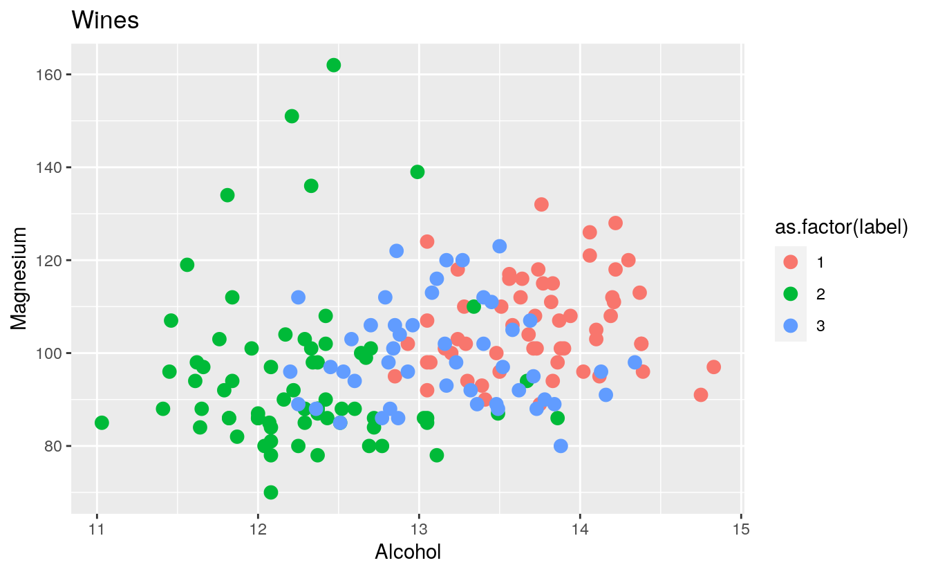
plt2 <- ggplot(wines, aes(x = Alcohol, y = Proline, colour = as.factor(label))) +
    geom_point(size=3) +
    ggtitle("Wines")
plt2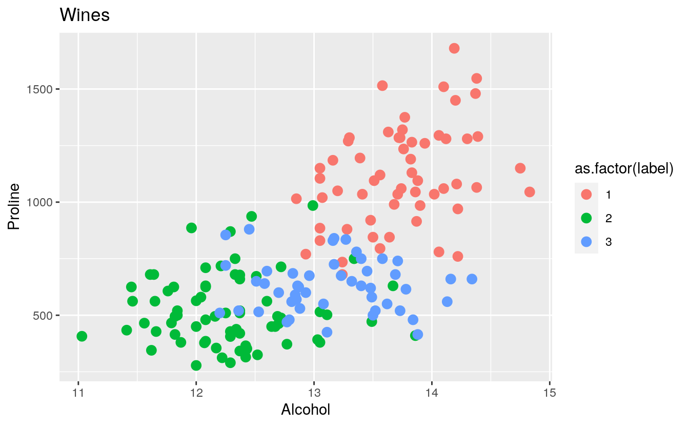
40.2 Preprocessing
During the preprocessing phase, I have to do at least the following two things:
Encode the categorical variables. Standardize the predictors. First of all, let’s encode our target variable. The encoding of the categorical variables is needed when using neuralnet since it does not like factors at all. It will shout at you if you try to feed in a factor (I am told nnet likes factors though).
In the wine dataset the variable label contains three different labels: 1,2 and 3.
The usual practice, as far as I know, is to encode categorical variables as a “one hot” vector. For instance, if I had three classes, like in this case, I’d need to replace the label variable with three variables like these:
#   l1,l2,l3
#   1,0,0
#   0,0,1
#   ...
In this case the first observation would be labeled as a 1, the second would be labeled as a 2, and so on. Ironically, the nnet package provides a function to perform this encoding in a painless way:
# Encode as a one hot vector multilabel data
train <- cbind(wines[, 2:14], class.ind(as.factor(wines$label)))

# Set labels name
names(train) <- c(names(wines)[2:14],"l1","l2","l3")
By the way, since the predictors are all continuous, you do not need to encode any of them, however, in case you needed to, you could apply the same strategy applied above to all the categorical predictors. Unless of course you’d like to try some other kind of custom encoding.
Now let’s standardize the predictors in the [0−1]">[0−1] interval by leveraging the lapply function:
# Scale data
scl <- function(x) { (x - min(x))/(max(x) - min(x)) }
train[, 1:13] <- data.frame(lapply(train[, 1:13], scl))
head(train)
#>   Alcohol Malic_acid   Ash Alcalinity_of_ash Magnesium Total_phenols Flavanoids
#> 1   0.571      0.206 0.417            0.0309     0.326         0.576      0.511
#> 2   0.561      0.320 0.701            0.4124     0.337         0.628      0.612
#> 3   0.879      0.239 0.610            0.3196     0.467         0.990      0.665
#> 4   0.582      0.366 0.807            0.5361     0.522         0.628      0.496
#> 5   0.834      0.202 0.583            0.2371     0.457         0.790      0.643
#> 6   0.884      0.223 0.583            0.2062     0.283         0.524      0.460
#>   Nonflavanoid_phenols Proanthocyanins Color_intensity   Hue
#> 1                0.245           0.274           0.265 0.463
#> 2                0.321           0.757           0.375 0.447
#> 3                0.208           0.558           0.556 0.309
#> 4                0.491           0.445           0.259 0.455
#> 5                0.396           0.492           0.467 0.463
#> 6                0.321           0.495           0.339 0.439
#>   OD280_OD315_of_diluted_wines Proline l1 l2 l3
#> 1                        0.780   0.551  1  0  0
#> 2                        0.696   0.647  1  0  0
#> 3                        0.799   0.857  1  0  0
#> 4                        0.608   0.326  1  0  0
#> 5                        0.579   0.836  1  0  0
#> 6                        0.846   0.722  1  0  0
40.3 Fitting the model with neuralnet
Now it is finally time to fit the model. As you might remember from the old post I wrote, neuralnet does not like the formula y~.. Fear not, you can build the formula to be used in a simple step:
# Set up formula
n <- names(train)
f <- as.formula(paste("l1 + l2 + l3 ~", paste(n[!n %in% c("l1","l2","l3")], collapse = " + ")))
f
#> l1 + l2 + l3 ~ Alcohol + Malic_acid + Ash + Alcalinity_of_ash +
#>     Magnesium + Total_phenols + Flavanoids + Nonflavanoid_phenols +
#>     Proanthocyanins + Color_intensity + Hue + OD280_OD315_of_diluted_wines +
#>     Proline
Note that the characters in the vector are not pasted to the right of the “~” symbol. Just remember to check that the formula is indeed correct and then you are good to go.
Let’s train the neural network with the full dataset. It should take very little time to converge. If you did not standardize the predictors it could take a lot more though.
nn <- neuralnet(f,
                data = train,
                hidden = c(13, 10, 3),
                act.fct = "logistic",
                linear.output = FALSE,
                lifesign = "minimal")
#> hidden: 13, 10, 3    thresh: 0.01    rep: 1/1    steps:      88  error: 0.03039  time: 0.05 secs
Note that I set the argument linear.output to FALSE in order to tell the model that I want to apply the activation function act.fct and that I am not doing a regression task. Then I set the activation function to logistic (which by the way is the default option) in order to apply the logistic function. The other available option is tanh but the model seems to perform a little worse with it so I opted for the default option. As far as I know these two are the only two available options, there is no relu function available although it seems to be a common activation function in other packages.
As far as the number of hidden neurons, I tried some combination and the one used seems to perform slightly better than the others (around 1% of accuracy difference in cross validation score).
By using the in-built plot method you can get a visual take on what is actually happening inside the model, however the plot is not that helpful I think
plot(nn)Let’s have a look at the accuracy on the training set:
# Compute predictions
pr.nn <- compute(nn, train[, 1:13])

# Extract results
pr.nn_ <- pr.nn$net.result
head(pr.nn_)
#>       [,1]    [,2]     [,3]
#> [1,] 0.990 0.00317 6.99e-06
#> [2,] 0.991 0.00233 8.69e-06
#> [3,] 0.991 0.00210 8.65e-06
#> [4,] 0.986 0.00442 8.74e-06
#> [5,] 0.992 0.00212 8.32e-06
#> [6,] 0.992 0.00214 8.34e-06
# Accuracy (training set)
original_values <- max.col(train[, 14:16])
pr.nn_2 <- max.col(pr.nn_)
mean(pr.nn_2 == original_values)
#> [1] 1
100% not bad! But wait, this may be because our model over fitted the data, furthermore evaluating accuracy on the training set is kind of cheating since the model already “knows” (or should know) the answers. In order to assess the “true accuracy” of the model you need to perform some kind of cross validation.
40.4 Cross validating the classifier
Let’s cross-validate the model using the evergreen 10 fold cross validation with the following train and test split: 95% of the dataset will be used as training set while the remaining 5% as test set.
Just out of curiosity, I decided to run a LOOCV round too. In case you’d like to run this cross validation technique, just set the proportion variable to 0.995: this will select just one observation for as test set and leave all the other observations as training set. Running LOOCV you should get similar results to the 10 fold cross validation.
# Set seed for reproducibility purposes
set.seed(500)
# 10 fold cross validation
k <- 10
# Results from cv
outs <- NULL
# Train test split proportions
proportion <- 0.95 # Set to 0.995 for LOOCV

# Crossvalidate, go!
for(i in 1:k)
{
    index <- sample(1:nrow(train), round(proportion*nrow(train)))
    train_cv <- train[index, ]
    test_cv <- train[-index, ]
    nn_cv <- neuralnet(f,
                        data = train_cv,
                        hidden = c(13, 10, 3),
                        act.fct = "logistic",
                        linear.output = FALSE)

    # Compute predictions
    pr.nn <- compute(nn_cv, test_cv[, 1:13])
    # Extract results
    pr.nn_ <- pr.nn$net.result
    # Accuracy (test set)
    original_values <- max.col(test_cv[, 14:16])
    pr.nn_2 <- max.col(pr.nn_)
    outs[i] <- mean(pr.nn_2 == original_values)
}

mean(outs)
#> [1] 0.978
98.8%, awesome! Next time when you are invited to a relaxing evening that includes a wine tasting competition I think you should definitely bring your laptop as a contestant!
Aside from that poor taste joke, (I made it again!), indeed this dataset is not the most challenging, I think with some more tweaking a better cross validation score could be achieved. Nevertheless I hope you found this tutorial useful. A gist with the entire code for this tutorial can be found here.
Thank you for reading this article, please feel free to leave a comment if you have any questions or suggestions and share the post with others if you find it useful.
Notes: