41.1 Introduction

Source: https://www.analyticsvidhya.com/blog/2017/09/creating-visualizing-neural-network-in-r/

Neural network is an information-processing machine and can be viewed as analogous to human nervous system. Just like human nervous system, which is made up of interconnected neurons, a neural network is made up of interconnected information processing units. The information processing units do not work in a linear manner. In fact, neural network draws its strength from parallel processing of information, which allows it to deal with non-linearity. Neural network becomes handy to infer meaning and detect patterns from complex data sets.

Neural network is considered as one of the most useful technique in the world of data analytics. However, it is complex and is often regarded as a black box, i.e. users view the input and output of a neural network but remain clueless about the knowledge generating process. We hope that the article will help readers learn about the internal mechanism of a neural network and get hands-on experience to implement it in R.

41.2 The Basics of Neural Networks

A neural network is a model characterized by an activation function, which is used by interconnected information processing units to transform input into output. A neural network has always been compared to human nervous system. Information in passed through interconnected units analogous to information passage through neurons in humans. The first layer of the neural network receives the raw input, processes it and passes the processed information to the hidden layers. The hidden layer passes the information to the last layer, which produces the output. The advantage of neural network is that it is adaptive in nature. It learns from the information provided, i.e. trains itself from the data, which has a known outcome and optimizes its weights for a better prediction in situations with unknown outcome.

A perceptron, viz. single layer neural network, is the most basic form of a neural network. A perceptron receives multidimensional input and processes it using a weighted summation and an activation function. It is trained using a labeled data and learning algorithm that optimize the weights in the summation processor. A major limitation of perceptron model is its inability to deal with non-linearity. A multilayered neural network overcomes this limitation and helps solve non-linear problems. The input layer connects with hidden layer, which in turn connects to the output layer. The connections are weighted and weights are optimized using a learning rule.

There are many learning rules that are used with neural network:

1. least mean square;
2. gradient descent;
3. newton’s rule;
4. conjugate gradient etc.

The learning rules can be used in conjunction with backpropgation error method. The learning rule is used to calculate the error at the output unit. This error is backpropagated to all the units such that the error at each unit is proportional to the contribution of that unit towards total error at the output unit. The errors at each unit are then used to optimize the weight at each connection. Figure 1 displays the structure of a simple neural network model for better understanding.

41.3 Fitting a Neural Network in R

Now we will fit a neural network model in R. In this article, we use a subset of cereal dataset shared by Carnegie Mellon University (CMU). The details of the dataset are on the following link: http://lib.stat.cmu.edu/DASL/Datafiles/Cereals.html. The objective is to predict rating of the cereals variables such as calories, proteins, fat etc. The R script is provided side by side and is commented for better understanding of the user. . The data is in .csv format and can be downloaded by clicking: cereals.

Please set working directory in R using setwd( ) function, and keep cereal.csv in the working directory. We use rating as the dependent variable and calories, proteins, fat, sodium and fiber as the independent variables. We divide the data into training and test set. Training set is used to find the relationship between dependent and independent variables while the test set assesses the performance of the model. We use 60% of the dataset as training set. The assignment of the data to training and test set is done using random sampling. We perform random sampling on R using sample ( ) function. We have used set.seed( ) to generate same random sample everytime and maintain consistency. We will use the index variable while fitting neural network to create training and test data sets. The R script is as follows:

## Creating index variable 

# Read the Data
data = read.csv(file.path(data_raw_dir, "cereals.csv"), header=T)

# Random sampling
samplesize = 0.60 * nrow(data)
set.seed(80)
index = sample( seq_len ( nrow ( data ) ), size = samplesize )

# Create training and test set  
datatrain = data[ index, ]
datatest = data[ -index, ]

dplyr::glimpse(data)
#> Rows: 75
#> Columns: 6
#> $ calories <int> 70, 120, 70, 50, 110, 110, 130, 90, 90, 120, 110, 120, 110, …
#> $ protein  <int> 4, 3, 4, 4, 2, 2, 3, 2, 3, 1, 6, 1, 3, 1, 2, 2, 1, 1, 3, 2, …
#> $ fat      <int> 1, 5, 1, 0, 2, 0, 2, 1, 0, 2, 2, 3, 2, 1, 0, 0, 0, 1, 3, 0, …
#> $ sodium   <int> 130, 15, 260, 140, 180, 125, 210, 200, 210, 220, 290, 210, 1…
#> $ fiber    <dbl> 10.0, 2.0, 9.0, 14.0, 1.5, 1.0, 2.0, 4.0, 5.0, 0.0, 2.0, 0.0…
#> $ rating   <dbl> 68.4, 34.0, 59.4, 93.7, 29.5, 33.2, 37.0, 49.1, 53.3, 18.0, …

Now we fit a neural network on our data. We use neuralnet library for the analysis. The first step is to scale the cereal dataset. The scaling of data is essential because otherwise a variable may have large impact on the prediction variable only because of its scale. Using unscaled may lead to meaningless results. The common techniques to scale data are: min-max normalization, Z-score normalization, median and MAD, and tan-h estimators. The min-max normalization transforms the data into a common range, thus removing the scaling effect from all the variables. Unlike Z-score normalization and median and MAD method, the min-max method retains the original distribution of the variables. We use min-max normalization to scale the data. The R script for scaling the data is as follows.

## Scale data for neural network

max = apply(data , 2 , max)
min = apply(data, 2 , min)
scaled = as.data.frame(scale(data, center = min, scale = max - min))

## Fit neural network 

# install library
# install.packages("neuralnet ")

# load library
library(neuralnet)

# creating training and test set
trainNN = scaled[index , ]
testNN = scaled[-index , ]

# fit neural network
set.seed(2)
NN = neuralnet(rating ~ calories + protein + fat + sodium + fiber, 
               trainNN, hidden = 3 , linear.output = T )

# plot neural network
plot(NN)

## Prediction using neural network

predict_testNN = compute(NN, testNN[,c(1:5)])
predict_testNN = (predict_testNN$net.result * (max(data$rating) - min(data$rating))) + min(data$rating)

plot(datatest$rating, predict_testNN, col='blue', pch=16, ylab = "predicted rating NN", xlab = "real rating")

abline(0,1)

# Calculate Root Mean Square Error (RMSE)
RMSE.NN = (sum((datatest$rating - predict_testNN)^2) / nrow(datatest)) ^ 0.5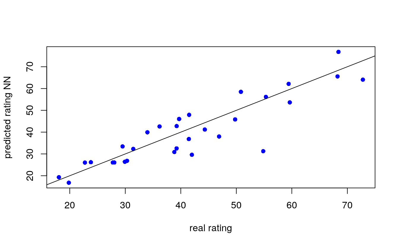

## Cross validation of neural network model

# install relevant libraries
# install.packages("boot")
# install.packages("plyr")

# Load libraries
library(boot)
library(plyr)

# Initialize variables
set.seed(50)
k = 100
RMSE.NN = NULL

List = list( )

# Fit neural network model within nested for loop
for(j in 10:65){
    for (i in 1:k) {
        index = sample(1:nrow(data),j )

        trainNN = scaled[index,]
        testNN = scaled[-index,]
        datatest = data[-index,]

        NN = neuralnet(rating ~ calories + protein + fat + sodium + fiber, trainNN, hidden = 3, linear.output= T)
        predict_testNN = compute(NN,testNN[,c(1:5)])
        predict_testNN = (predict_testNN$net.result*(max(data$rating)-min(data$rating)))+min(data$rating)

        RMSE.NN [i]<- (sum((datatest$rating - predict_testNN)^2)/nrow(datatest))^0.5
    }
    List[[j]] = RMSE.NN
}

Matrix.RMSE = do.call(cbind, List)

## Prepare boxplot
boxplot(Matrix.RMSE[,56], ylab = "RMSE", main = "RMSE BoxPlot (length of traning set = 65)")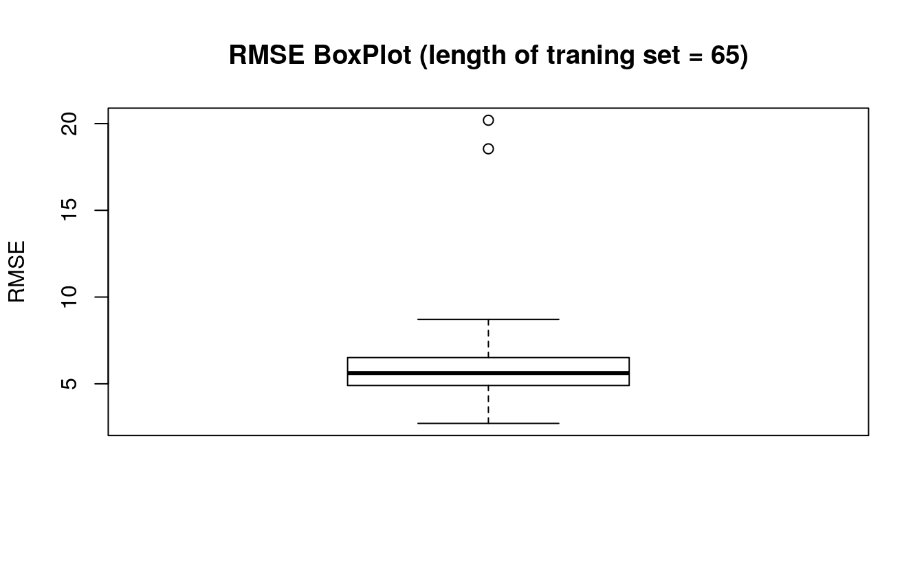

## Variation of median RMSE 
# install.packages("matrixStats")
library(matrixStats)
#> 
#> Attaching package: 'matrixStats'
#> The following object is masked from 'package:plyr':
#> 
#>     count

med = colMedians(Matrix.RMSE)

X = seq(10,65)

plot (med~X, type = "l", xlab = "length of training set", ylab = "median RMSE", main = "Variation of RMSE with length of training set")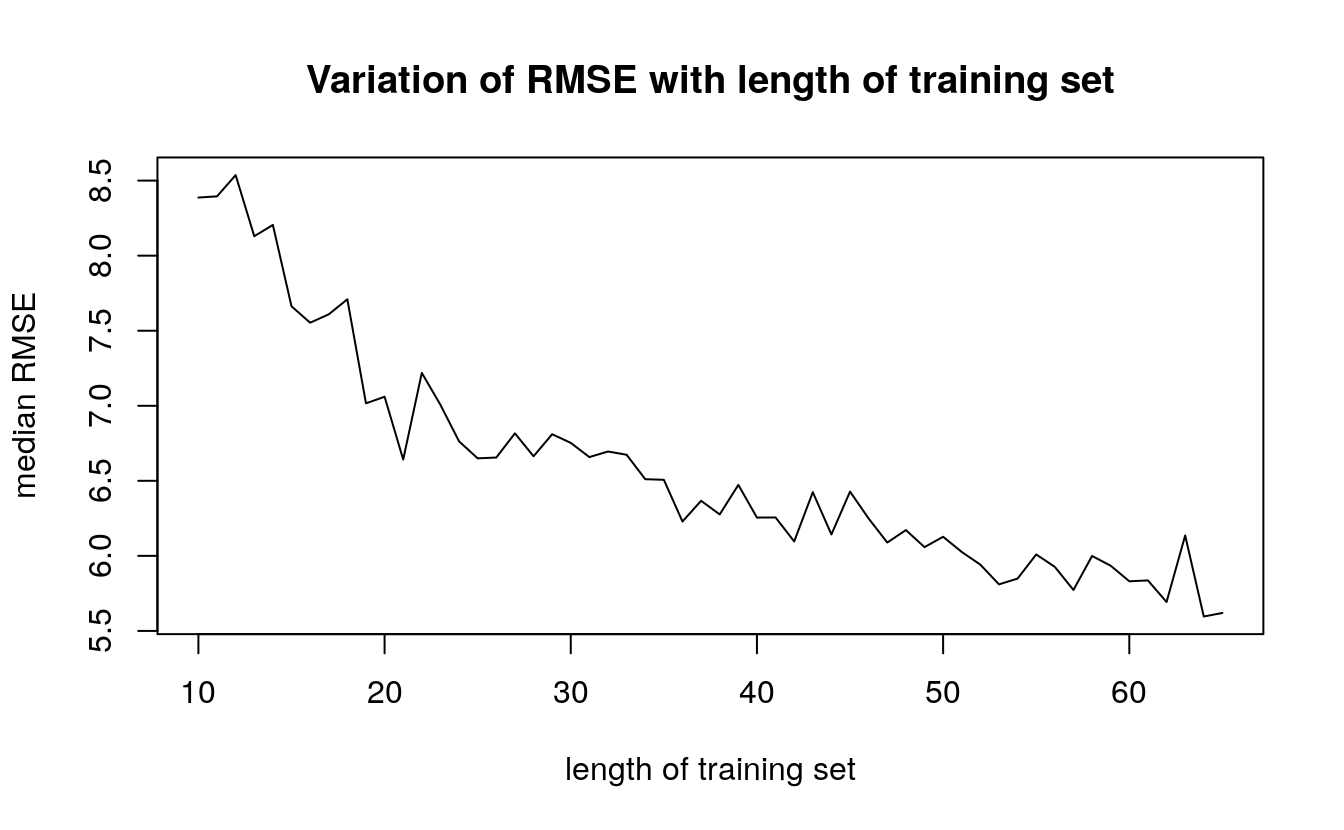

Figure 41.1: Variation of RMSE

Figure 41.1) shows that the median RMSE of our model decreases as the length of the training the set. This is an important result. The reader must remember that the model accuracy is dependent on the length of training set. The performance of neural network model is sensitive to training-test split.

41.4 End Notes

The article discusses the theoretical aspects of a neural network, its implementation in R and post training evaluation. A Neural network is inspired from biological nervous system. Similar to nervous system the information is passed through layers of processors. The significance of variables is represented by weights of each connection. The article provides basic understanding of back propagation algorithm, which is used to assign these weights. In this article we also implement neural network on R. We use a publicly available dataset shared by CMU. The aim is to predict the rating of cereals using information such as calories, fat, protein etc. After constructing the neural network we evaluate the model for accuracy and robustness. We compute RMSE and perform cross-validation analysis. In cross validation, we check the variation in model accuracy as the length of training set is changed. We consider training sets with length 10 to 65. For each length a 100 samples are random picked and median RMSE is calculated. We show that model accuracy increases when training set is large. Before using the model for prediction, it is important to check the robustness of performance through cross validation.

The article provides a quick review neural network and is a useful reference for data enthusiasts. We have provided commented R code throughout the article to help readers with hands on experience of using neural networks.