4.1 Data standardization

In principal component analysis, variables are often scaled ( i.e. standardized). This is particularly recommended when variables are measured in different scales (e.g: kilograms, kilometers, centimeters, …); otherwise, the PCA outputs obtained will be severely affected.

The goal is to make the variables comparable. Generally variables are scaled to have i) standard deviation one and ii) mean zero.

The function PCA() [FactoMineR package] can be used. A simplified format is:

library(FactoMineR)
res.pca <- PCA(decathlon2.active, graph = FALSE)

print(res.pca)
#> **Results for the Principal Component Analysis (PCA)**
#> The analysis was performed on 23 individuals, described by 10 variables
#> *The results are available in the following objects:
#> 
#>    name               description                          
#> 1  "$eig"             "eigenvalues"                        
#> 2  "$var"             "results for the variables"          
#> 3  "$var$coord"       "coord. for the variables"           
#> 4  "$var$cor"         "correlations variables - dimensions"
#> 5  "$var$cos2"        "cos2 for the variables"             
#> 6  "$var$contrib"     "contributions of the variables"     
#> 7  "$ind"             "results for the individuals"        
#> 8  "$ind$coord"       "coord. for the individuals"         
#> 9  "$ind$cos2"        "cos2 for the individuals"           
#> 10 "$ind$contrib"     "contributions of the individuals"   
#> 11 "$call"            "summary statistics"                 
#> 12 "$call$centre"     "mean of the variables"              
#> 13 "$call$ecart.type" "standard error of the variables"    
#> 14 "$call$row.w"      "weights for the individuals"        
#> 15 "$call$col.w"      "weights for the variables"

The object that is created using the function PCA() contains many information found in many different lists and matrices. These values are described in the next section.

4.2 Eigenvalues / Variances

As described in previous sections, the eigenvalues measure the amount of variation retained by each principal component. Eigenvalues are large for the first PCs and small for the subsequent PCs. That is, the first PCs corresponds to the directions with the maximum amount of variation in the data set.

We examine the eigenvalues to determine the number of principal components to be considered. The eigenvalues and the proportion of variances (i.e., information) retained by the principal components (PCs) can be extracted using the function get_eigenvalue() [factoextra package].

library(factoextra)
eig.val <- get_eigenvalue(res.pca)
eig.val
#>        eigenvalue variance.percent cumulative.variance.percent
#> Dim.1       4.124            41.24                        41.2
#> Dim.2       1.839            18.39                        59.6
#> Dim.3       1.239            12.39                        72.0
#> Dim.4       0.819             8.19                        80.2
#> Dim.5       0.702             7.02                        87.2
#> Dim.6       0.423             4.23                        91.5
#> Dim.7       0.303             3.03                        94.5
#> Dim.8       0.274             2.74                        97.2
#> Dim.9       0.155             1.55                        98.8
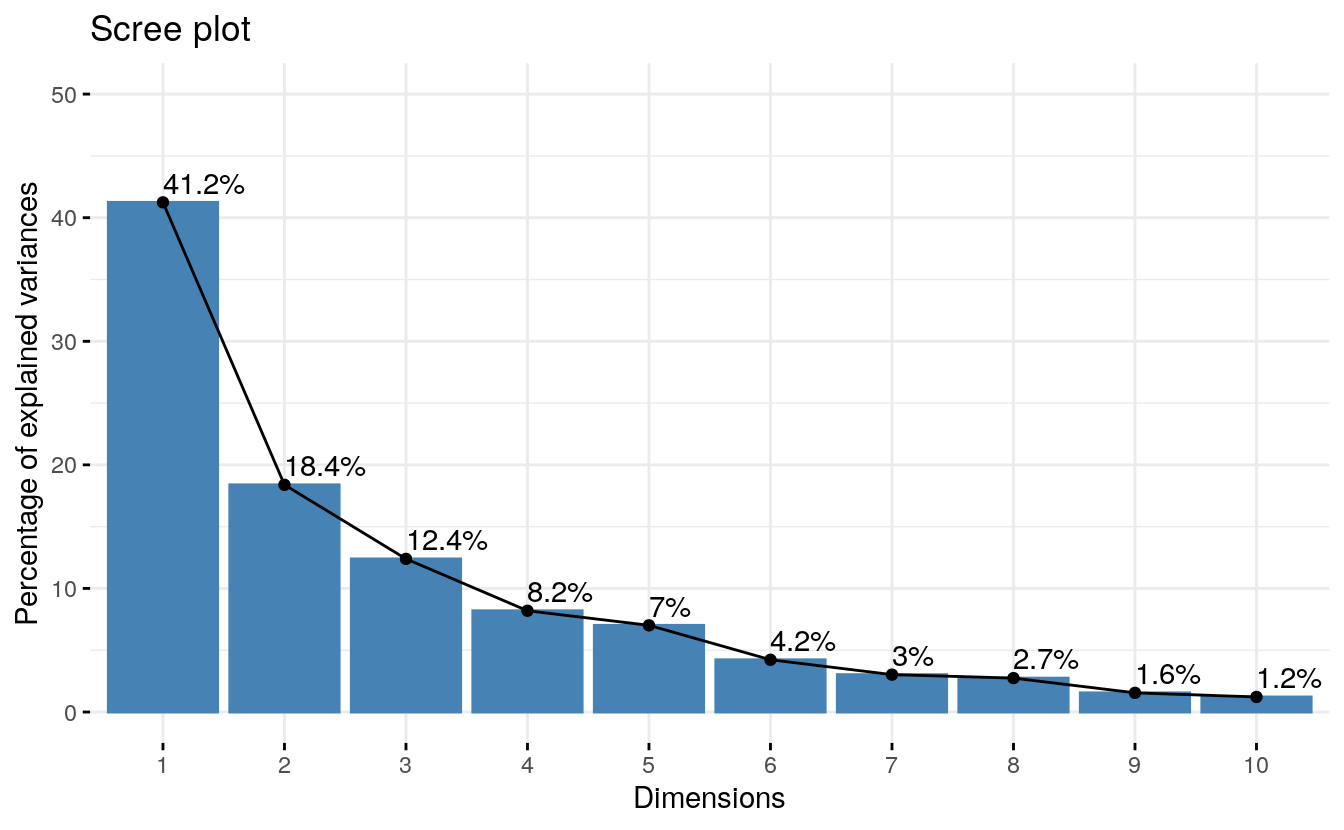
#> Dim.10      0.122             1.22                       100.0

The sum of all the eigenvalues give a total variance of 10.

The proportion of variation explained by each eigenvalue is given in the second column. For example, 4.124 divided by 10 equals 0.4124, or, about 41.24% of the variation is explained by this first eigenvalue. The cumulative percentage explained is obtained by adding the successive proportions of variation explained to obtain the running total. For instance, 41.242% plus 18.385% equals 59.627%, and so forth. Therefore, about 59.627% of the variation is explained by the first two eigenvalues together.

Unfortunately, there is no well-accepted objective way to decide how many principal components are enough. This will depend on the specific field of application and the specific data set. In practice, we tend to look at the first few principal components in order to find interesting patterns in the data.

In our analysis, the first three principal components explain 72% of the variation. This is an acceptably large percentage.

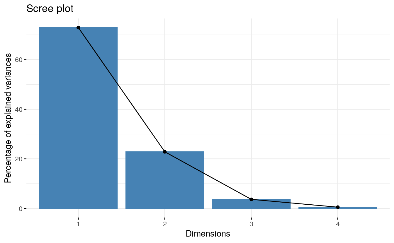
An alternative method to determine the number of principal components is to look at a Scree Plot, which is the plot of eigenvalues ordered from largest to the smallest. The number of component is determined at the point, beyond which the remaining eigenvalues are all relatively small and of comparable size (Jollife 2002, Peres-Neto, Jackson, and Somers (2005)).

The scree plot can be produced using the function fviz_eig() or fviz_screeplot() [factoextra package].

fviz_eig(res.pca, addlabels = TRUE, ylim = c(0, 50))

From the plot above, we might want to stop at the fifth principal component. 87% of the information (variances) contained in the data are retained by the first five principal components.

4.3 Graph of variables

Results A simple method to extract the results, for variables, from a PCA output is to use the function get_pca_var() [factoextra package]. This function provides a list of matrices containing all the results for the active variables (coordinates, correlation between variables and axes, squared cosine and contributions)

var <- get_pca_var(res.pca)
var
#> Principal Component Analysis Results for variables
#>  ===================================================
#>   Name       Description                                    
#> 1 "$coord"   "Coordinates for the variables"                
#> 2 "$cor"     "Correlations between variables and dimensions"
#> 3 "$cos2"    "Cos2 for the variables"                       
#> 4 "$contrib" "contributions of the variables"

The components of the get_pca_var() can be used in the plot of variables as follow:

• var$coord: coordinates of variables to create a scatter plot
• var$cos2: represents the quality of representation for variables on the factor map. It’s calculated as the squared coordinates: var.cos2 = var.coord * var.coord.
• var$contrib: contains the contributions (in percentage) of the variables to the principal components. The contribution of a variable (var) to a given principal component is (in percentage) : (var.cos2 * 100) / (total cos2 of the component).

Note that, it’s possible to plot variables and to color them according to either i) their quality on the factor map (cos2) or ii) their contribution values to the principal components (contrib).

The different components can be accessed as follow:

# Coordinates
head(var$coord)
#>               Dim.1   Dim.2  Dim.3   Dim.4  Dim.5
#> X100m        -0.851 -0.1794  0.302  0.0336 -0.194
#> Long.jump     0.794  0.2809 -0.191 -0.1154  0.233
#> Shot.put      0.734  0.0854  0.518  0.1285 -0.249
#> High.jump     0.610 -0.4652  0.330  0.1446  0.403
#> X400m        -0.702  0.2902  0.284  0.4308  0.104
#> X110m.hurdle -0.764 -0.0247  0.449 -0.0169  0.224
# Cos2: quality on the factore map
head(var$cos2)
#>              Dim.1    Dim.2  Dim.3    Dim.4  Dim.5
#> X100m        0.724 0.032184 0.0909 0.001127 0.0378
#> Long.jump    0.631 0.078881 0.0363 0.013315 0.0544
#> Shot.put     0.539 0.007294 0.2679 0.016504 0.0619
#> High.jump    0.372 0.216424 0.1090 0.020895 0.1622
#> X400m        0.492 0.084203 0.0804 0.185611 0.0108
#> X110m.hurdle 0.584 0.000612 0.2015 0.000285 0.0503
# Contributions to the principal components
head(var$contrib)
#>              Dim.1   Dim.2 Dim.3   Dim.4 Dim.5
#> X100m        17.54  1.7505  7.34  0.1376  5.39
#> Long.jump    15.29  4.2904  2.93  1.6249  7.75
#> Shot.put     13.06  0.3967 21.62  2.0141  8.82
#> High.jump     9.02 11.7716  8.79  2.5499 23.12
#> X400m        11.94  4.5799  6.49 22.6509  1.54
#> X110m.hurdle 14.16  0.0333 16.26  0.0348  7.17

In this section, we describe how to visualize variables and draw conclusions about their correlations. Next, we highlight variables according to either i) their quality of representation on the factor map or ii) their contributions to the principal components.

4.4 Correlation circle

The correlation between a variable and a principal component (PC) is used as the coordinates of the variable on the PC. The representation of variables differs from the plot of the observations: The observations are represented by their projections, but the variables are represented by their correlations (Abdi and Williams 2010).

# Coordinates of variables
head(var$coord, 4)
#>            Dim.1   Dim.2  Dim.3   Dim.4  Dim.5
#> X100m     -0.851 -0.1794  0.302  0.0336 -0.194
#> Long.jump  0.794  0.2809 -0.191 -0.1154  0.233
#> Shot.put   0.734  0.0854  0.518  0.1285 -0.249
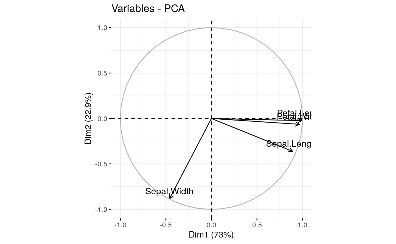
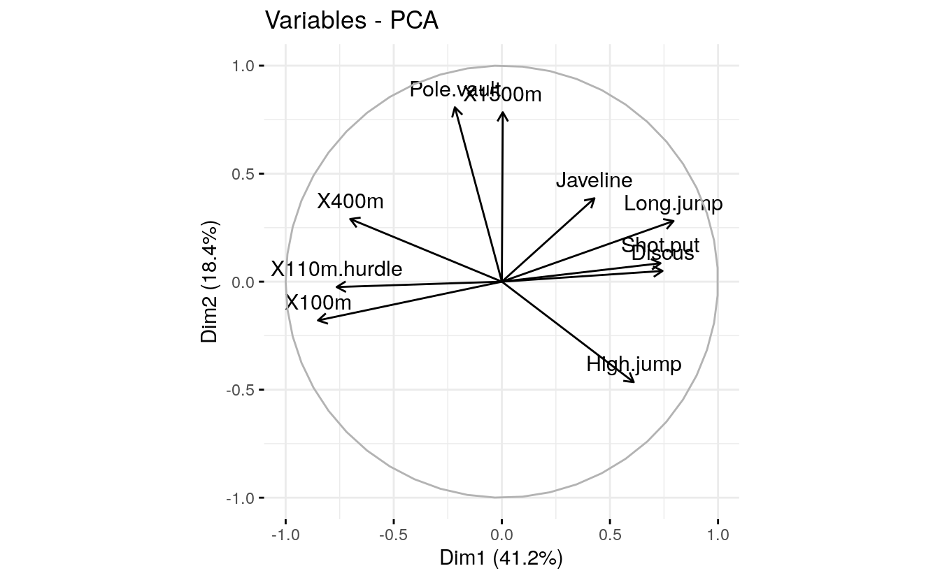
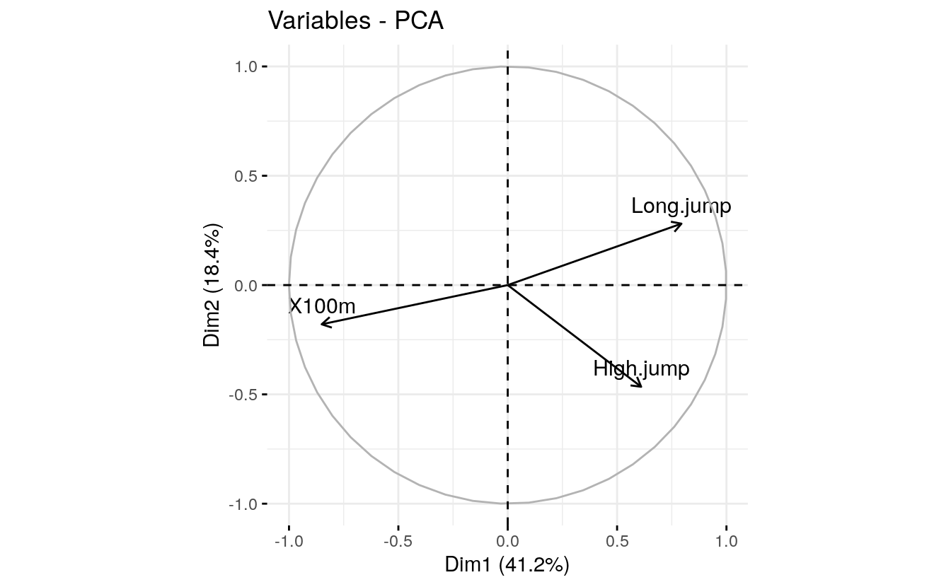
#> High.jump  0.610 -0.4652  0.330  0.1446  0.403

To plot variables, type this:

fviz_pca_var(res.pca, col.var = "black")

The plot above is also known as variable correlation plots. It shows the relationships between all variables. It can be interpreted as follow:

• Positively correlated variables are grouped together.
• Negatively correlated variables are positioned on opposite sides of the plot origin (opposed quadrants).
• The distance between variables and the origin measures the quality of the variables on the factor map. Variables that are away from the origin are well represented on the factor map.

4.5 Quality of representation

The quality of representation of the variables on factor map is called cos2 (square cosine, squared coordinates) . You can access to the cos2 as follow:

head(var$cos2, 4)
#>           Dim.1   Dim.2  Dim.3   Dim.4  Dim.5
#> X100m     0.724 0.03218 0.0909 0.00113 0.0378
#> Long.jump 0.631 0.07888 0.0363 0.01331 0.0544
#> Shot.put  0.539 0.00729 0.2679 0.01650 0.0619
#> High.jump 0.372 0.21642 0.1090 0.02089 0.1622

You can visualize the cos2 of variables on all the dimensions using the corrplot package:

library(corrplot)
#> corrplot 0.84 loaded
corrplot(var$cos2, is.corr=FALSE)

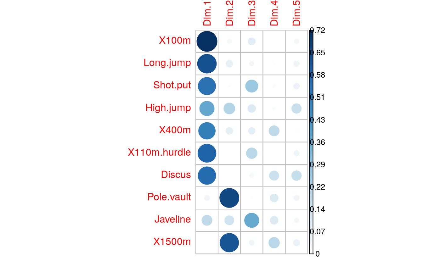
It’s also possible to create a bar plot of variables cos2 using the function fviz_cos2() [in factoextra]:

# Total cos2 of variables on Dim.1 and Dim.2
fviz_cos2(res.pca, choice = "var", axes = 1:2)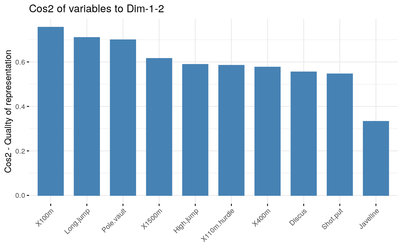

Note that,

• A high cos2 indicates a good representation of the variable on the principal component. In this case the variable is positioned close to the circumference of the correlation circle.

• A low cos2 indicates that the variable is not perfectly represented by the PCs. In this case the variable is close to the center of the circle.

For a given variable, the sum of the cos2 on all the principal components is equal to one.

If a variable is perfectly represented by only two principal components (Dim.1 & Dim.2), the sum of the cos2 on these two PCs is equal to one. In this case the variables will be positioned on the circle of correlations.

For some of the variables, more than 2 components might be required to perfectly represent the data. In this case the variables are positioned inside the circle of correlations.

In summary:

• The cos2 values are used to estimate the quality of the representation
• The closer a variable is to the circle of correlations, the better its representation on the factor map (and the more important it is to interpret these components)
• Variables that are closed to the center of the plot are less important for the first components.

It’s possible to color variables by their cos2 values using the argument col.var = "cos2". This produces a gradient colors. In this case, the argument gradient.cols can be used to provide a custom color. For instance, gradient.cols = c(“white”, “blue”, “red”) means that:

• variables with low cos2 values will be colored in “white”
• variables with mid cos2 values will be colored in “blue”
• variables with high cos2 values will be colored in red

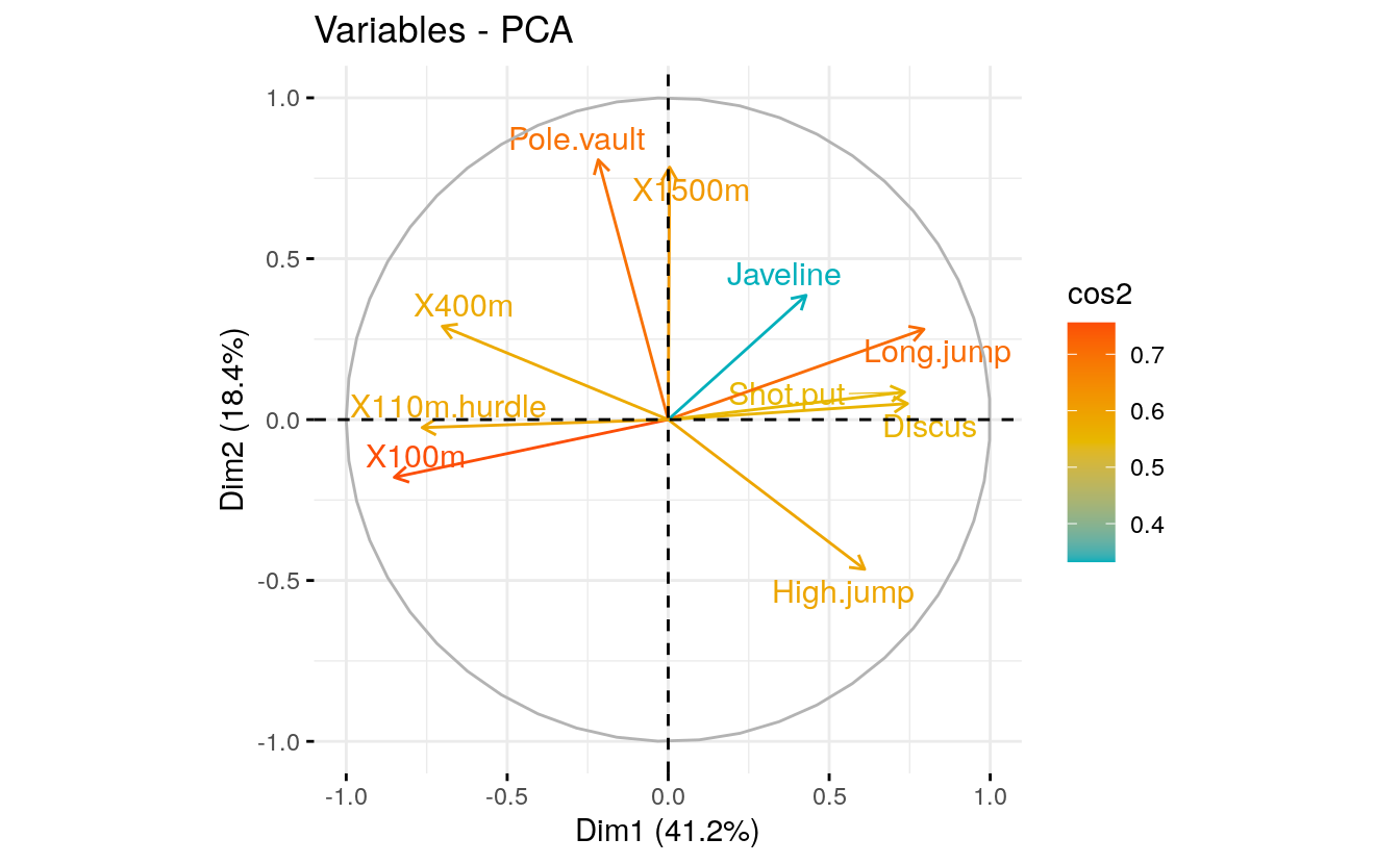
# Color by cos2 values: quality on the factor map
fviz_pca_var(res.pca, col.var = "cos2",
             gradient.cols = c("#00AFBB", "#E7B800", "#FC4E07"), 
             repel = TRUE # Avoid text overlapping
             )

Note that, it’s also possible to change the transparency of the variables according to their cos2 values using the option alpha.var = “cos2”. For example, type this:

# Change the transparency by cos2 values
fviz_pca_var(res.pca, alpha.var = "cos2")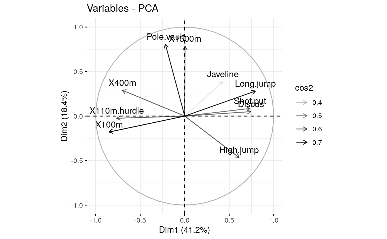

4.6 Contributions of variables to PCs

The contributions of variables in accounting for the variability in a given principal component are expressed in percentage.

• Variables that are correlated with PC1 (i.e., Dim.1) and PC2 (i.e., Dim.2) are the most important in explaining the variability in the data set.
• Variables that do not correlated with any PC or correlated with the last dimensions are variables with low contribution and might be removed to simplify the overall analysis.

The contribution of variables can be extracted as follow :

head(var$contrib, 4)
#>           Dim.1  Dim.2 Dim.3 Dim.4 Dim.5
#> X100m     17.54  1.751  7.34 0.138  5.39
#> Long.jump 15.29  4.290  2.93 1.625  7.75
#> Shot.put  13.06  0.397 21.62 2.014  8.82
#> High.jump  9.02 11.772  8.79 2.550 23.12

The larger the value of the contribution, the more the variable contributes to the component.

It’s possible to use the function corrplot() [corrplot package] to highlight the most contributing variables for each dimension:

library("corrplot")

corrplot(var$contrib, is.corr=FALSE)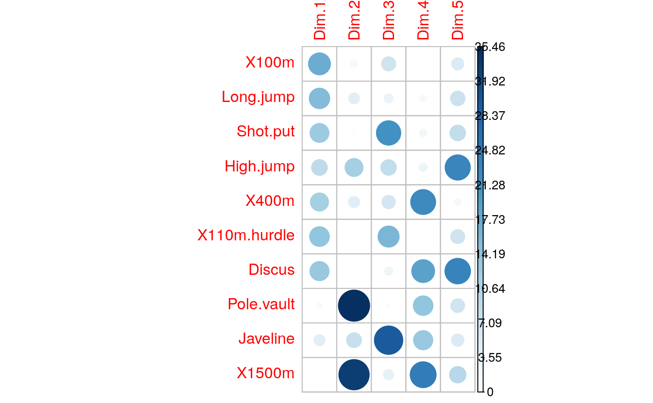    

The function fviz_contrib() [factoextra package] can be used to draw a bar plot of variable contributions. If your data contains many variables, you can decide to show only the top contributing variables. The R code below shows the top 10 variables contributing to the principal components:

# Contributions of variables to PC1
fviz_contrib(res.pca, choice = "var", axes = 1, top = 10)
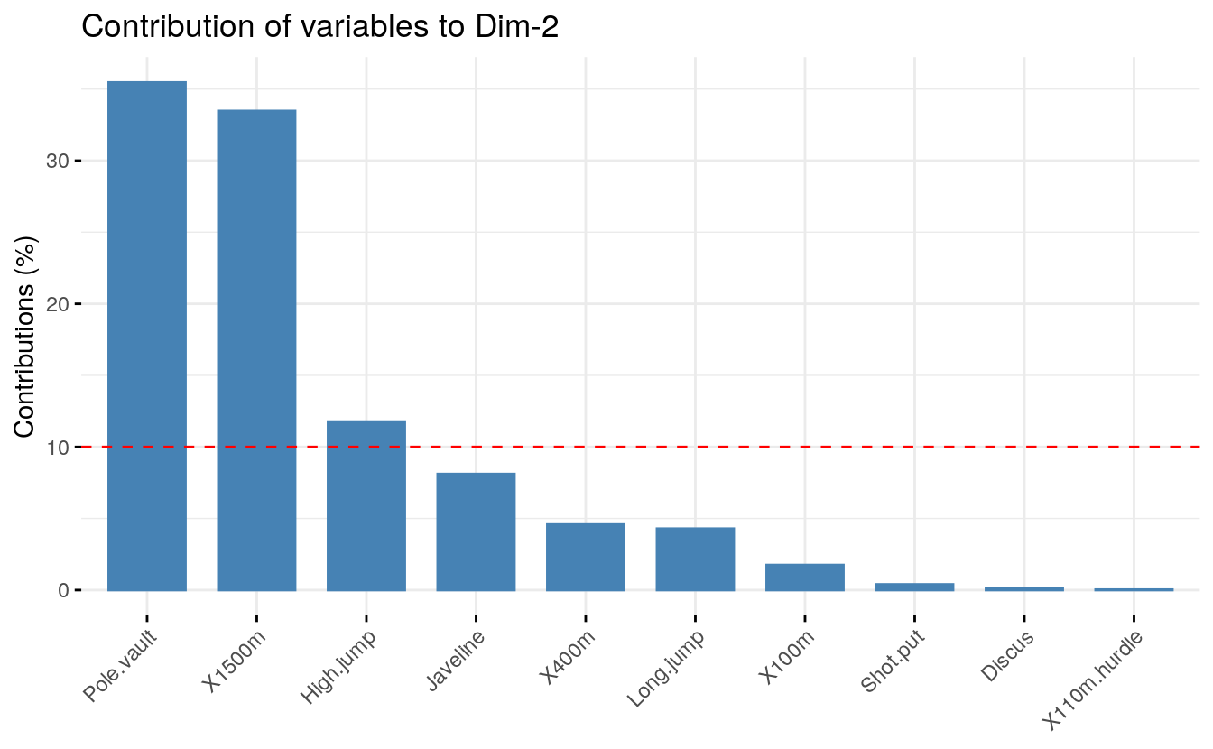
# Contributions of variables to PC2
fviz_contrib(res.pca, choice = "var", axes = 2, top = 10)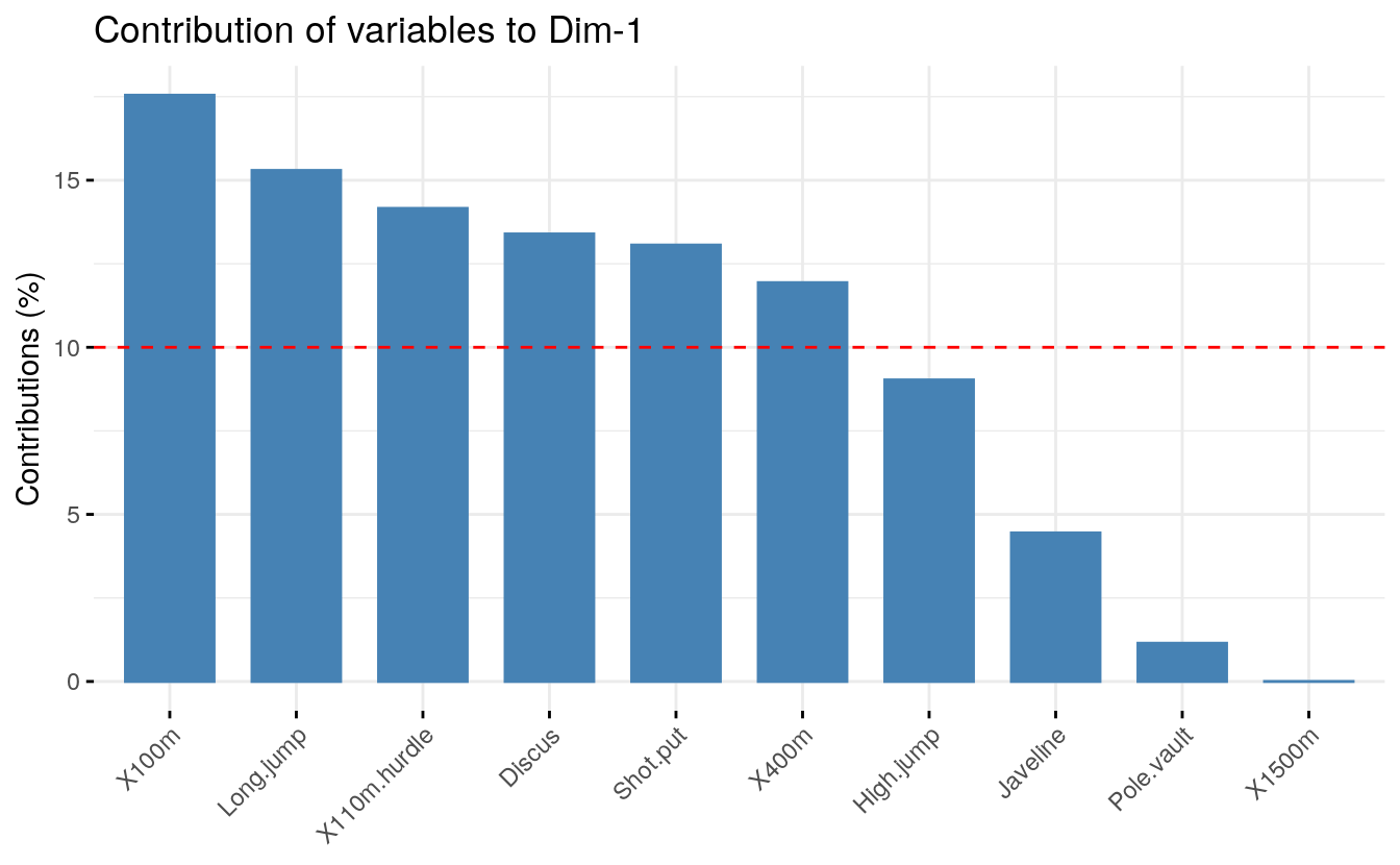

The total contribution to PC1 and PC2 is obtained with the following R code:

fviz_contrib(res.pca, choice = "var", axes = 1:2, top = 10)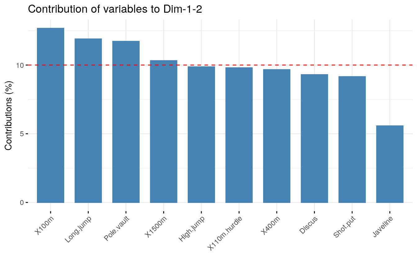

The red dashed line on the graph above indicates the expected average contribution. If the contribution of the variables were uniform, the expected value would be 1/length(variables) = 1/10 = 10%. For a given component, a variable with a contribution larger than this cutoff could be considered as important in contributing to the component.

Note that, the total contribution of a given variable, on explaining the variations retained by two principal components, say PC1 and PC2, is calculated as contrib = [(C1 * Eig1) + (C2 * Eig2)]/(Eig1 + Eig2), where

• C1 and C2 are the contributions of the variable on PC1 and PC2, respectively
• Eig1 and Eig2 are the eigenvalues of PC1 and PC2, respectively. Recall that eigenvalues measure the amount of variation retained by each PC.

In this case, the expected average contribution (cutoff) is calculated as follow: As mentioned above, if the contributions of the 10 variables were uniform, the expected average contribution on a given PC would be 1/10 = 10%. The expected average contribution of a variable for PC1 and PC2 is : [(10* Eig1) + (10 * Eig2)]/(Eig1 + Eig2)

It can be seen that the variables - X100m, Long.jump and Pole.vault - contribute the most to the dimensions 1 and 2.

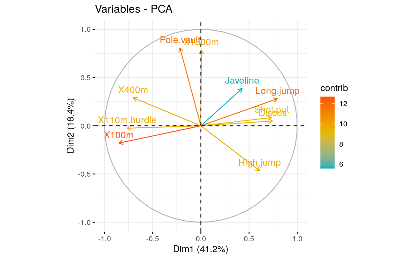
The most important (or, contributing) variables can be highlighted on the correlation plot as follow:

fviz_pca_var(res.pca, col.var = "contrib",
             gradient.cols = c("#00AFBB", "#E7B800", "#FC4E07")
             )

Note that, it’s also possible to change the transparency of variables according to their contrib values using the option alpha.var = "contrib". For example, type this:

# Change the transparency by contrib values
fviz_pca_var(res.pca, alpha.var = "contrib")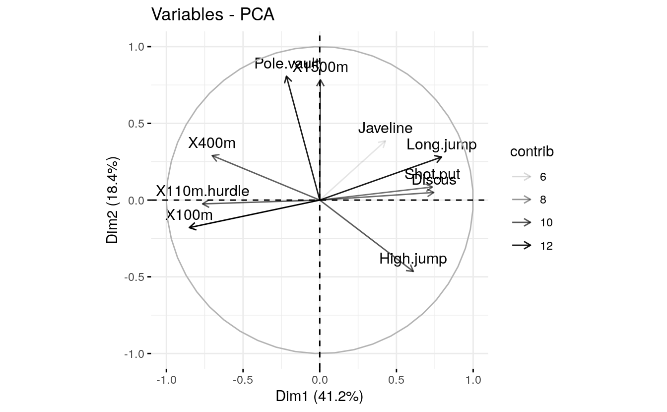

4.7 Color by a custom continuous variable

In the previous sections, we showed how to color variables by their contributions and their cos2. Note that, it’s possible to color variables by any custom continuous variable. The coloring variable should have the same length as the number of active variables in the PCA (here n = 10).

For example, type this:

# Create a random continuous variable of length 10
set.seed(123)
my.cont.var <- rnorm(10)
# Color variables by the continuous variable
fviz_pca_var(res.pca, col.var = my.cont.var,
             gradient.cols = c("blue", "yellow", "red"),
             legend.title = "Cont.Var")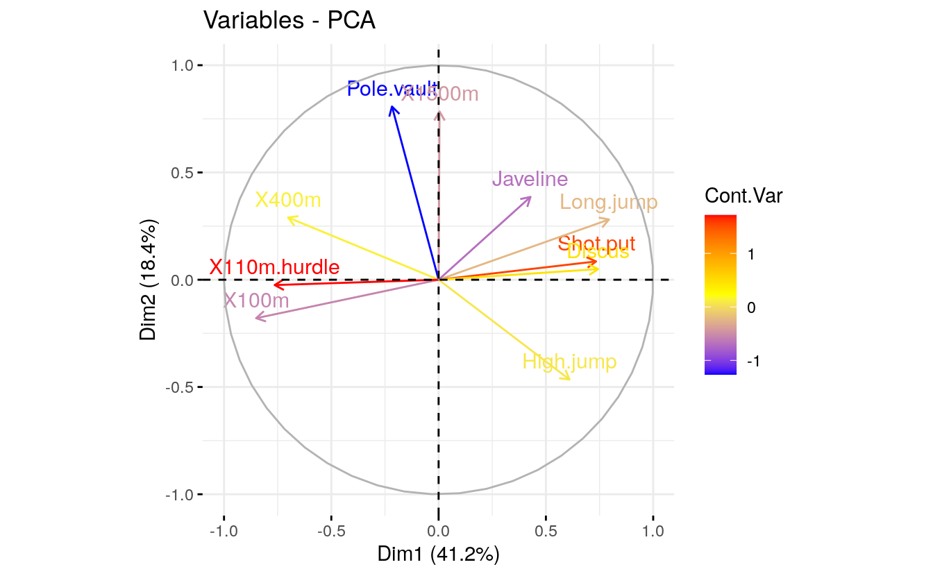

4.8 Color by groups

It’s also possible to change the color of variables by groups defined by a qualitative/categorical variable, also called factor in R terminology.

As we don’t have any grouping variable in our data sets for classifying variables, we’ll create it.

In the following demo example, we start by classifying the variables into 3 groups using the kmeans clustering algorithm. Next, we use the clusters returned by the kmeans algorithm to color variables.

# Create a grouping variable using kmeans
# Create 3 groups of variables (centers = 3)
set.seed(123)
res.km <- kmeans(var$coord, centers = 3, nstart = 25)
grp <- as.factor(res.km$cluster)
# Color variables by groups
fviz_pca_var(res.pca, col.var = grp, 
             palette = c("#0073C2FF", "#EFC000FF", "#868686FF"),
             legend.title = "Cluster")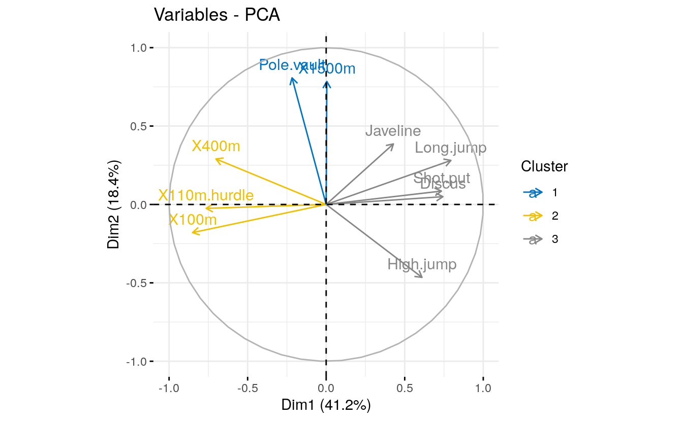

4.9 Dimension description

In the section (???)(pca-variable-contributions), we described how to highlight variables according to their contributions to the principal components.

Note also that, the function dimdesc() [in FactoMineR], for dimension description, can be used to identify the most significantly associated variables with a given principal component . It can be used as follow:

res.desc <- dimdesc(res.pca, axes = c(1,2), proba = 0.05)
# Description of dimension 1
res.desc$Dim.1
#> $quanti
#>              correlation  p.value
#> Long.jump          0.794 6.06e-06
#> Discus             0.743 4.84e-05
#> Shot.put           0.734 6.72e-05
#> High.jump          0.610 1.99e-03
#> Javeline           0.428 4.15e-02
#> X400m             -0.702 1.91e-04
#> X110m.hurdle      -0.764 2.20e-05
#> X100m             -0.851 2.73e-07
#> 
#> attr(,"class")
#> [1] "condes" "list "

# Description of dimension 2
res.desc$Dim.2
#> $quanti
#>            correlation  p.value
#> Pole.vault       0.807 3.21e-06
#> X1500m           0.784 9.38e-06
#> High.jump       -0.465 2.53e-02
#> 
#> attr(,"class")
#> [1] "condes" "list "

4.10 Graph of individuals

Results The results, for individuals can be extracted using the function get_pca_ind()[factoextra package]. Similarly to the get_pca_var(), the function get_pca_ind() provides a list of matrices containing all the results for the individuals (coordinates, correlation between individuals and axes, squared cosine and contributions)

ind <- get_pca_ind(res.pca)
ind
#> Principal Component Analysis Results for individuals
#>  ===================================================
#>   Name       Description                       
#> 1 "$coord"   "Coordinates for the individuals" 
#> 2 "$cos2"    "Cos2 for the individuals"        
#> 3 "$contrib" "contributions of the individuals"

To get access to the different components, use this:

# Coordinates of individuals
head(ind$coord)
#>            Dim.1  Dim.2  Dim.3   Dim.4   Dim.5
#> SEBRLE     0.196  1.589  0.642  0.0839  1.1683
#> CLAY       0.808  2.475 -1.387  1.2984 -0.8250
#> BERNARD   -1.359  1.648  0.201 -1.9641  0.0842
#> YURKOV    -0.889 -0.443  2.530  0.7129  0.4078
#> ZSIVOCZKY -0.108 -2.069 -1.334 -0.1015 -0.2015
#> McMULLEN   0.121 -1.014 -0.863  1.3416  1.6215
# Quality of individuals
head(ind$cos2)
#>             Dim.1  Dim.2   Dim.3   Dim.4    Dim.5
#> SEBRLE    0.00753 0.4975 0.08133 0.00139 0.268903
#> CLAY      0.04870 0.4570 0.14363 0.12579 0.050785
#> BERNARD   0.19720 0.2900 0.00429 0.41182 0.000757
#> YURKOV    0.09611 0.0238 0.77823 0.06181 0.020228
#> ZSIVOCZKY 0.00157 0.5764 0.23975 0.00139 0.005465
#> McMULLEN  0.00218 0.1522 0.11014 0.26649 0.389262
# Contributions of individuals
head(ind$contrib)
#>            Dim.1  Dim.2  Dim.3   Dim.4   Dim.5
#> SEBRLE    0.0403  5.971  1.448  0.0373  8.4589
#> CLAY      0.6881 14.484  6.754  8.9446  4.2179
#> BERNARD   1.9474  6.423  0.141 20.4682  0.0439
#> YURKOV    0.8331  0.463 22.452  2.6966  1.0308
#> ZSIVOCZKY 0.0123 10.122  6.246  0.0547  0.2515
#> McMULLEN  0.0155  2.431  2.610  9.5506 16.2949

4.11 Plots: quality and contribution

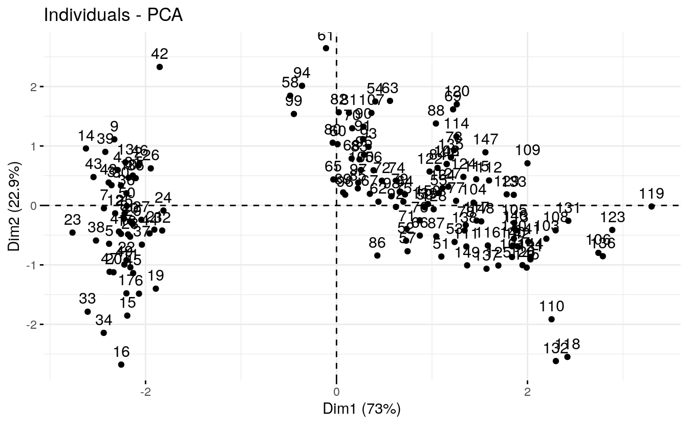
The fviz_pca_ind() is used to produce the graph of individuals. To create a simple plot, type this:

fviz_pca_ind(res.pca)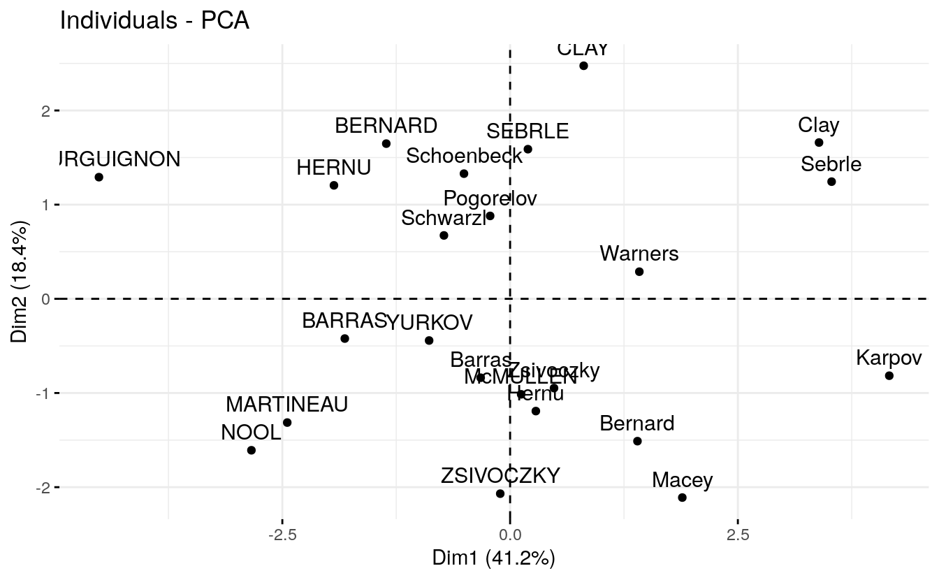

Like variables, it’s also possible to color individuals by their cos2 values:

fviz_pca_ind(res.pca, col.ind = "cos2", 
             gradient.cols = c("#00AFBB", "#E7B800", "#FC4E07"),
             repel = TRUE # Avoid text overlapping (slow if many points)
             )

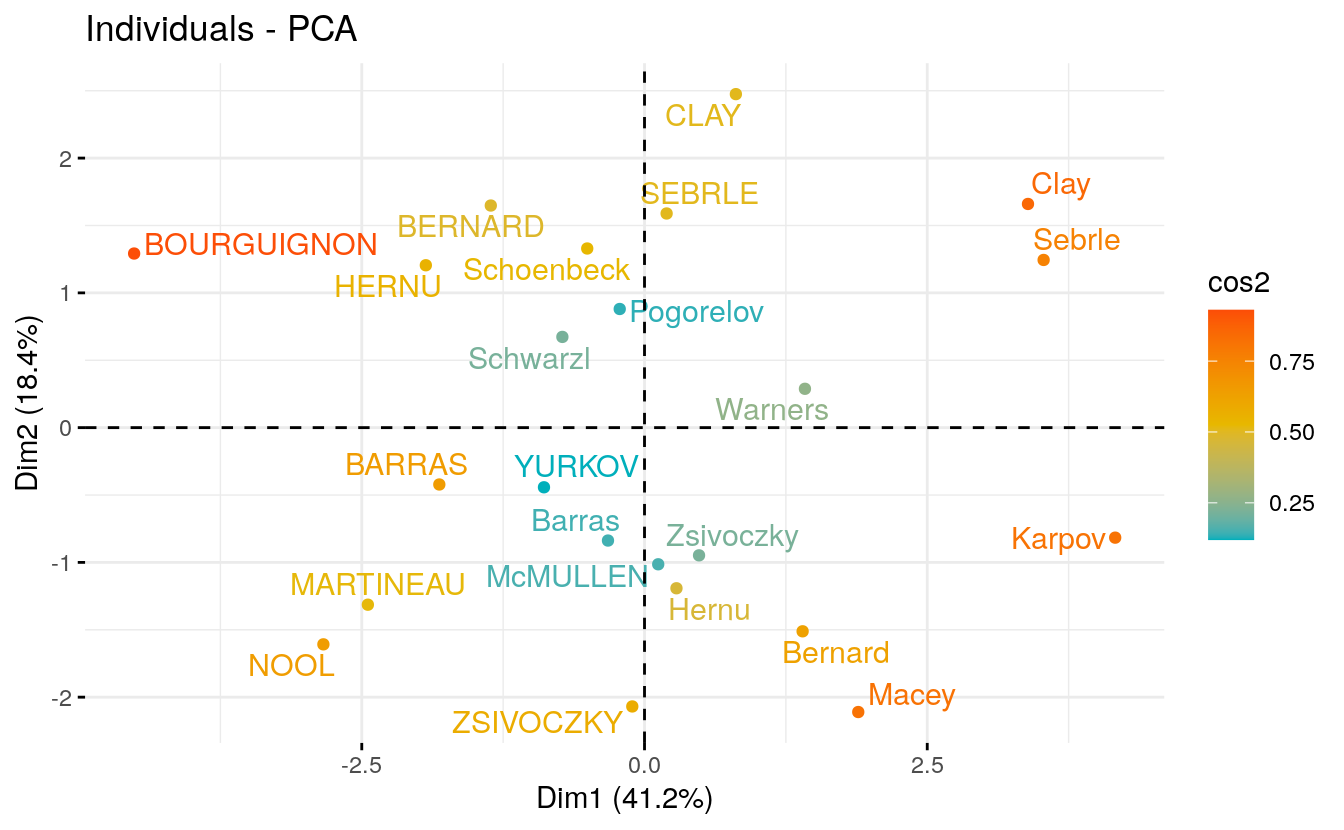
Note that, individuals that are similar are grouped together on the plot.

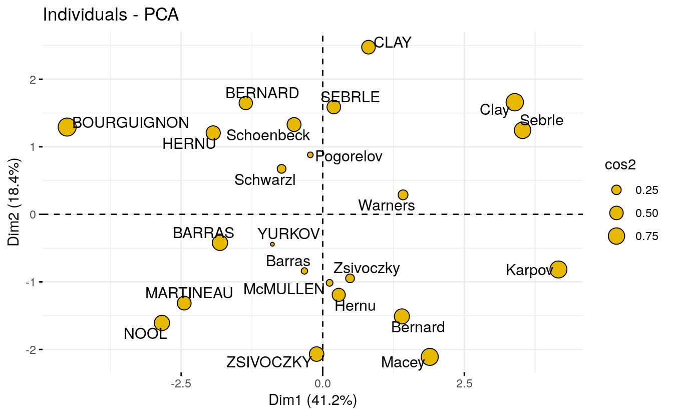
You can also change the point size according the cos2 of the corresponding individuals:

fviz_pca_ind(res.pca, pointsize = "cos2", 
             pointshape = 21, fill = "#E7B800",
             repel = TRUE # Avoid text overlapping (slow if many points)
             )

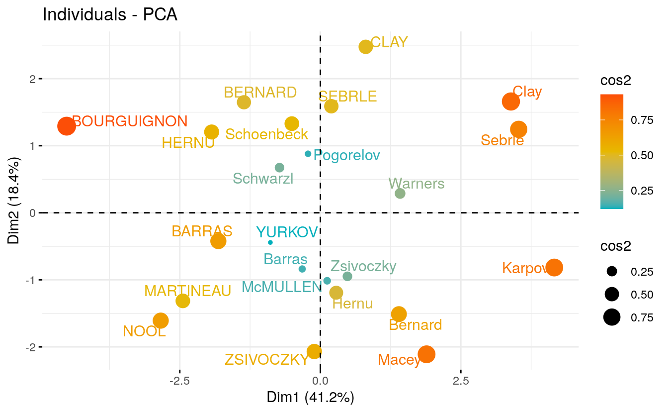
To change both point size and color by cos2, try this:

fviz_pca_ind(res.pca, col.ind = "cos2", pointsize = "cos2",
             gradient.cols = c("#00AFBB", "#E7B800", "#FC4E07"),
             repel = TRUE # Avoid text overlapping (slow if many points)
             )

To create a bar plot of the quality of representation (cos2) of individuals on the factor map, you can use the function fviz_cos2() as previously described for variables:

fviz_cos2(res.pca, choice = "ind")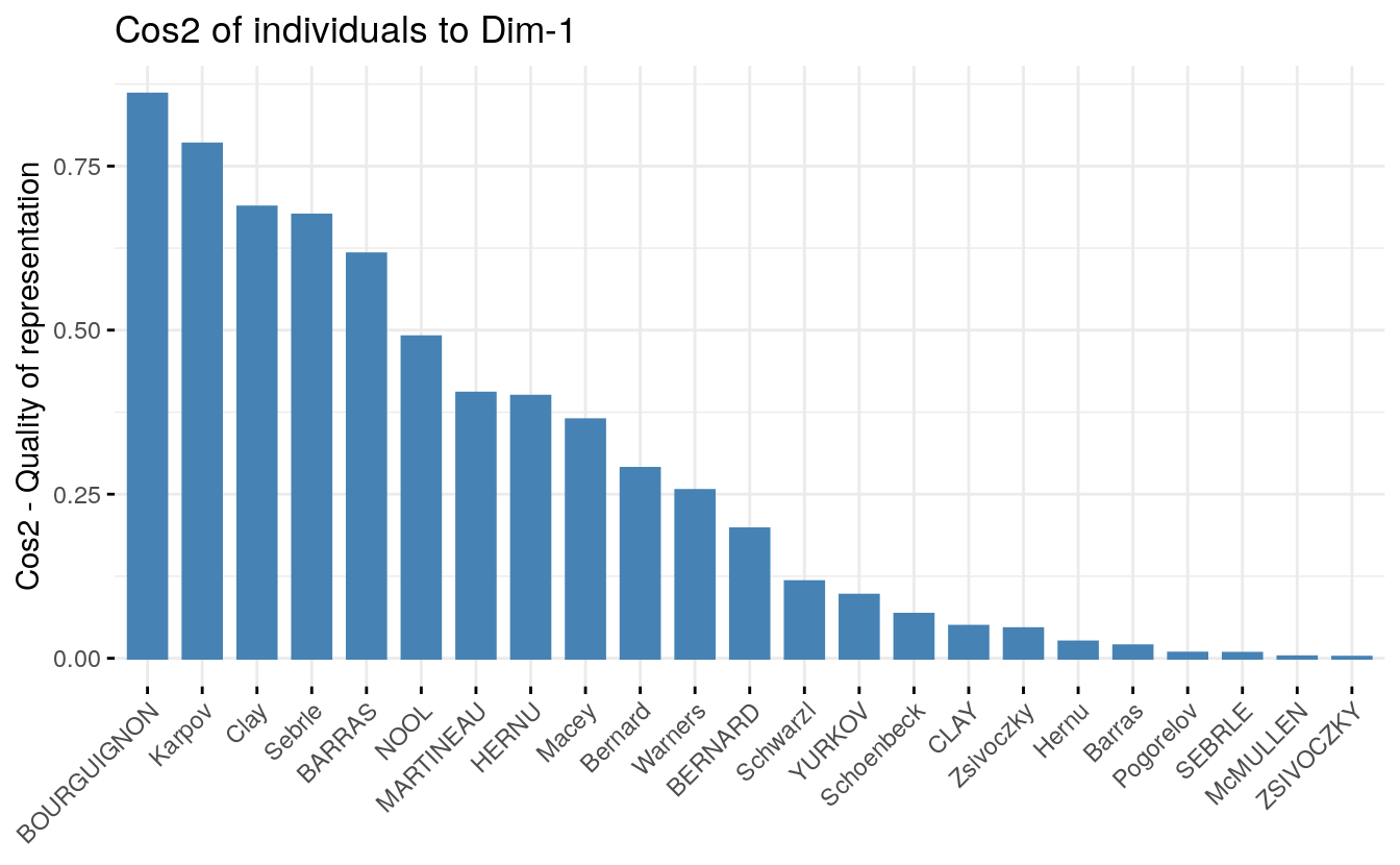

To visualize the contribution of individuals to the first two principal components, type this:

# Total contribution on PC1 and PC2
fviz_contrib(res.pca, choice = "ind", axes = 1:2)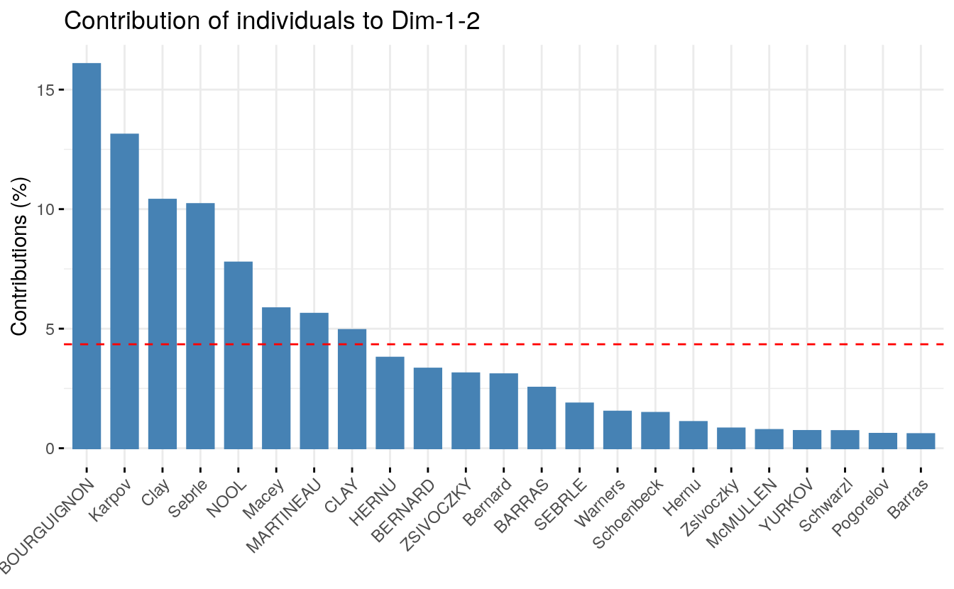

4.12 Color by a custom continuous variable

As for variables, individuals can be colored by any custom continuous variable by specifying the argument col.ind.

For example, type this:

# Create a random continuous variable of length 23,
# Same length as the number of active individuals in the PCA
set.seed(123)
my.cont.var <- rnorm(23)
# Color individuals by the continuous variable
fviz_pca_ind(res.pca, col.ind = my.cont.var,
             gradient.cols = c("blue", "yellow", "red"),
             legend.title = "Cont.Var")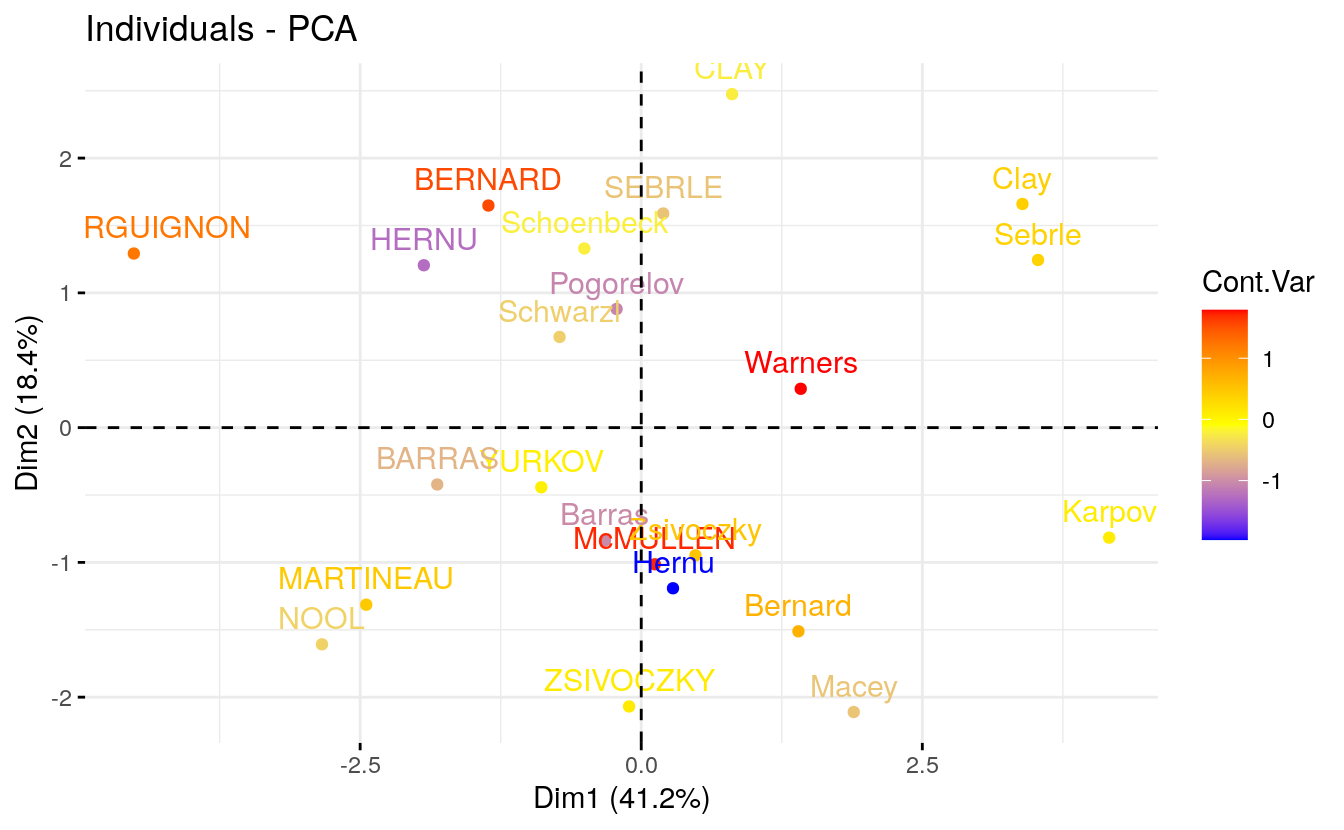

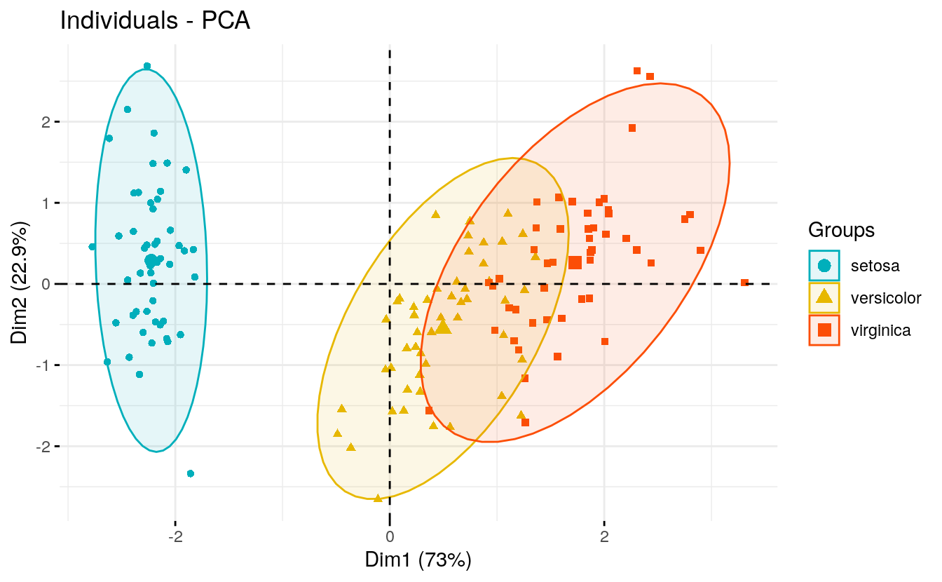
4.13 Color by groups

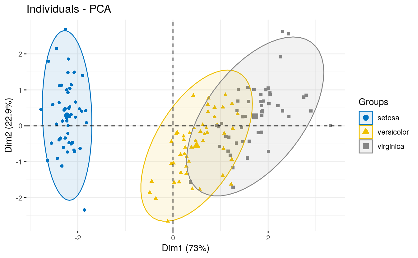
Here, we describe how to color individuals by group. Additionally, we show how to add concentration ellipses and confidence ellipses by groups. For this, we’ll use the iris data as demo data sets.

Iris data sets look like this:

head(iris, 3)
#>   Sepal.Length Sepal.Width Petal.Length Petal.Width Species
#> 1          5.1         3.5          1.4         0.2  setosa
#> 2          4.9         3.0          1.4         0.2  setosa
#> 3          4.7         3.2          1.3         0.2  setosa

The column “Species” will be used as grouping variable. We start by computing principal component analysis as follow:

# The variable Species (index = 5) is removed
# before PCA analysis
iris.pca <- PCA(iris[,-5], graph = FALSE)

In the R code below: the argument habillage or col.ind can be used to specify the factor variable for coloring the individuals by groups.

To add a concentration ellipse around each group, specify the argument addEllipses = TRUE. The argument palette can be used to change group colors.

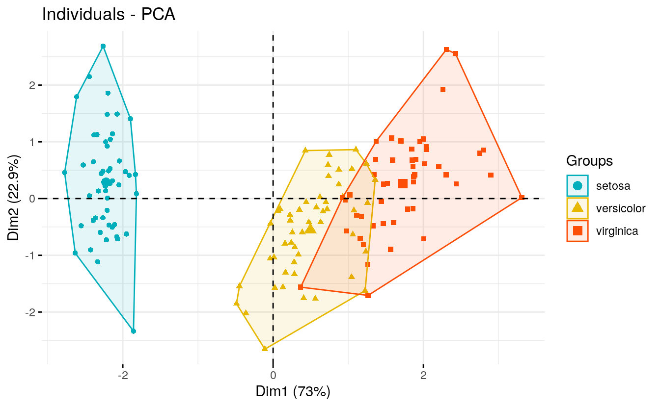
fviz_pca_ind(iris.pca,
             geom.ind = "point", # show points only (nbut not "text")
             col.ind = iris$Species, # color by groups
             palette = c("#00AFBB", "#E7B800", "#FC4E07"),
             addEllipses = TRUE, # Concentration ellipses
             legend.title = "Groups"
             )

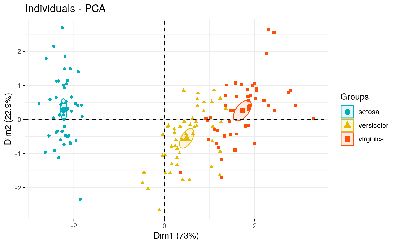
To remove the group mean point, specify the argument mean.point = FALSE. If you want confidence ellipses instead of concentration ellipses, use ellipse.type = “confidence”.

# Add confidence ellipses
fviz_pca_ind(iris.pca, geom.ind = "point", col.ind = iris$Species, 
             palette = c("#00AFBB", "#E7B800", "#FC4E07"),
             addEllipses = TRUE, ellipse.type = "confidence",
             legend.title = "Groups"
             )

Note that, allowed values for palette include:

• “grey” for grey color palettes;
• brewer palettes e.g. “RdBu”, “Blues”, …; To view all, type this in R: RColorBrewer::display.brewer.all().
• custom color palette e.g. c(“blue”, “red”); and scientific journal palettes from ggsci R package, e.g.: “npg”, “aaas”, * “lancet”, “jco”, “ucscgb”, “uchicago”, “simpsons” and “rickandmorty”. For example, to use the jco (journal of clinical oncology) color palette, type this:

fviz_pca_ind(iris.pca,
             label = "none", # hide individual labels
             habillage = iris$Species, # color by groups
             addEllipses = TRUE, # Concentration ellipses
             palette = "jco"
             )

4.14 Graph customization

Note that, fviz_pca_ind() and fviz_pca_var() and related functions are wrapper around the core function fviz() [in factoextra]. fviz() is a wrapper around the function ggscatter() [in ggpubr]. Therefore, further arguments, to be passed to the function fviz() and ggscatter(), can be specified in fviz_pca_ind() and fviz_pca_var().

Here, we present some of these additional arguments to customize the PCA graph of variables and individuals.

4.14.1 Dimensions

By default, variables/individuals are represented on dimensions 1 and 2. If you want to visualize them on dimensions 2 and 3, for example, you should specify the argument axes = c(2, 3).

# Variables on dimensions 2 and 3
fviz_pca_var(res.pca, axes = c(2, 3))
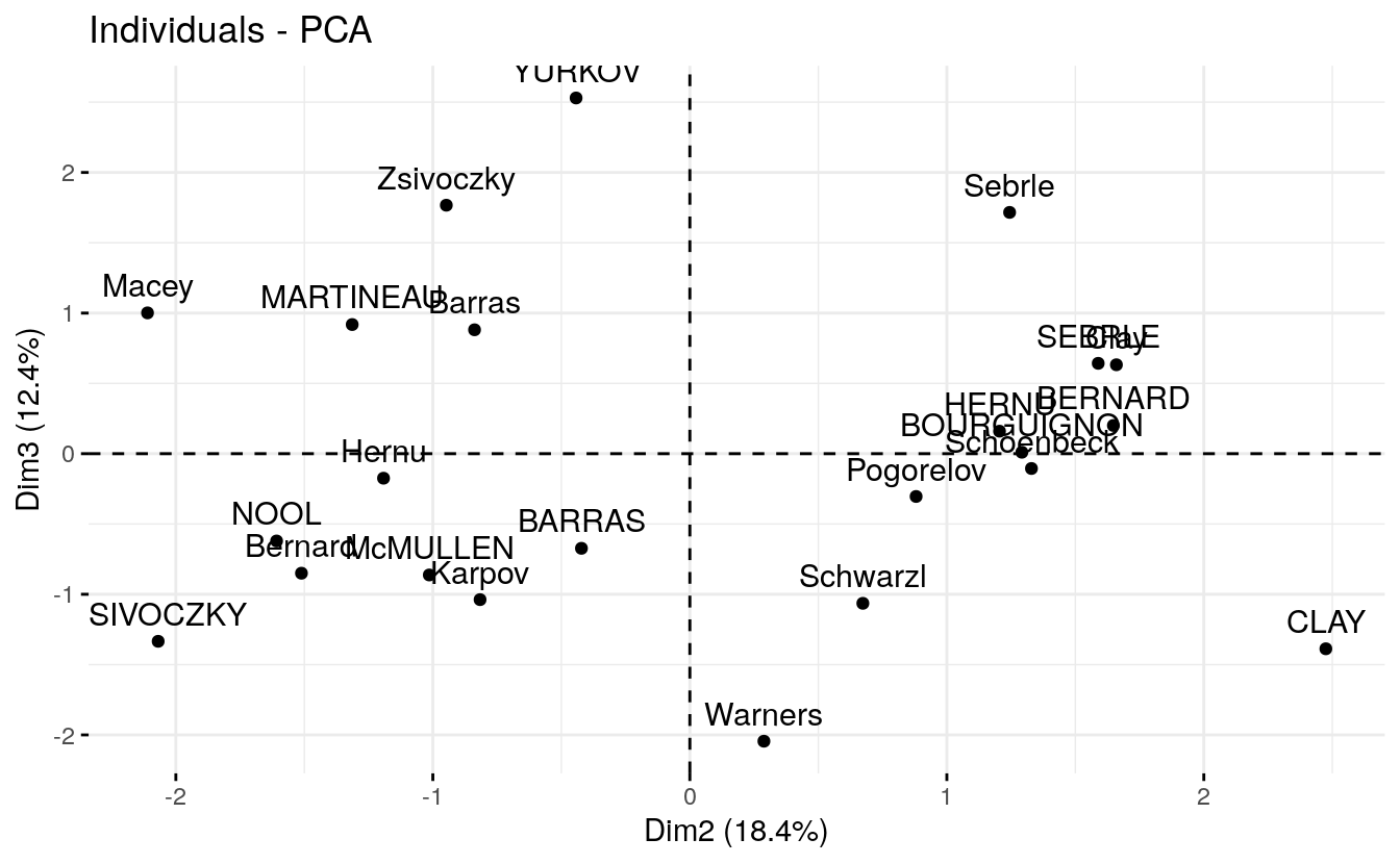
# Individuals on dimensions 2 and 3
fviz_pca_ind(res.pca, axes = c(2, 3))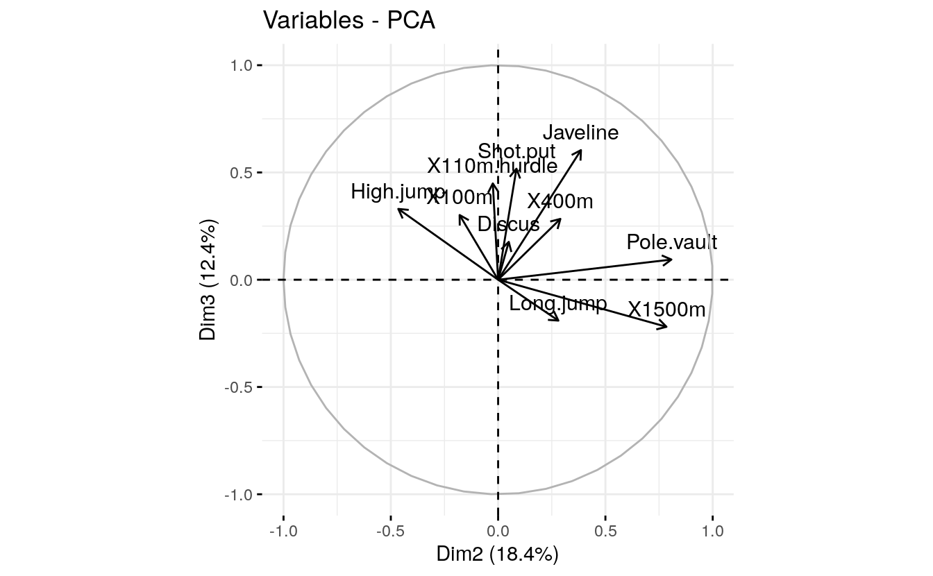

Plot elements: point, text, arrow The argument geom (for geometry) and derivatives are used to specify the geometry elements or graphical elements to be used for plotting.

1. geom.var: a text specifying the geometry to be used for plotting variables. Allowed values are the combination of c(“point”, “arrow”, “text”).

• Use geom.var = “point”, to show only points;
• Use geom.var = “text” to show only text labels;
• Use geom.var = c(“point”, “text”) to show both points and text labels
• Use geom.var = c(“arrow”, “text”) to show arrows and labels (default).

For example, type this:

# Show variable points and text labels
fviz_pca_var(res.pca, geom.var = c("point", "text"))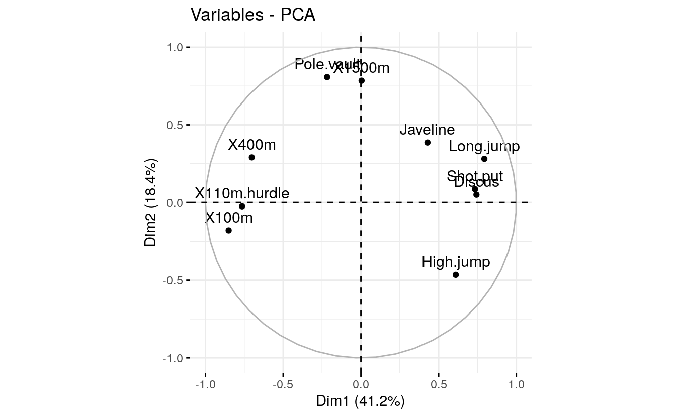

# Show individuals text labels only
fviz_pca_ind(res.pca, geom.ind =  "text")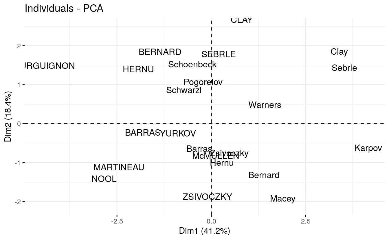

4.15 Size and shape of plot elements

# Change the size of arrows an labels
fviz_pca_var(res.pca, arrowsize = 1, labelsize = 5, 
             repel = TRUE)
# Change points size, shape and fill color
# Change labelsize
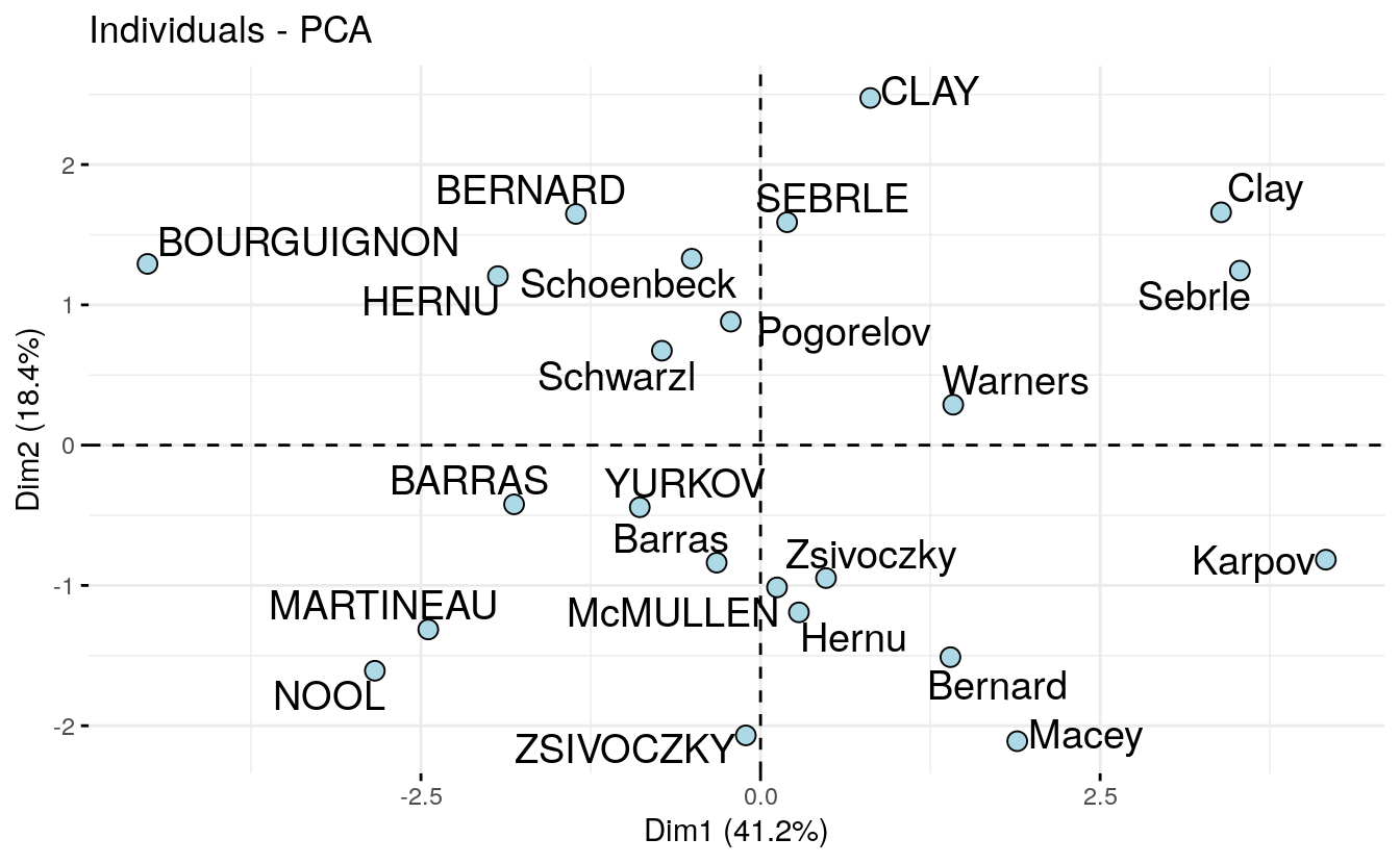
fviz_pca_ind(res.pca, 
             pointsize = 3, pointshape = 21, fill = "lightblue",
             labelsize = 5, repel = TRUE)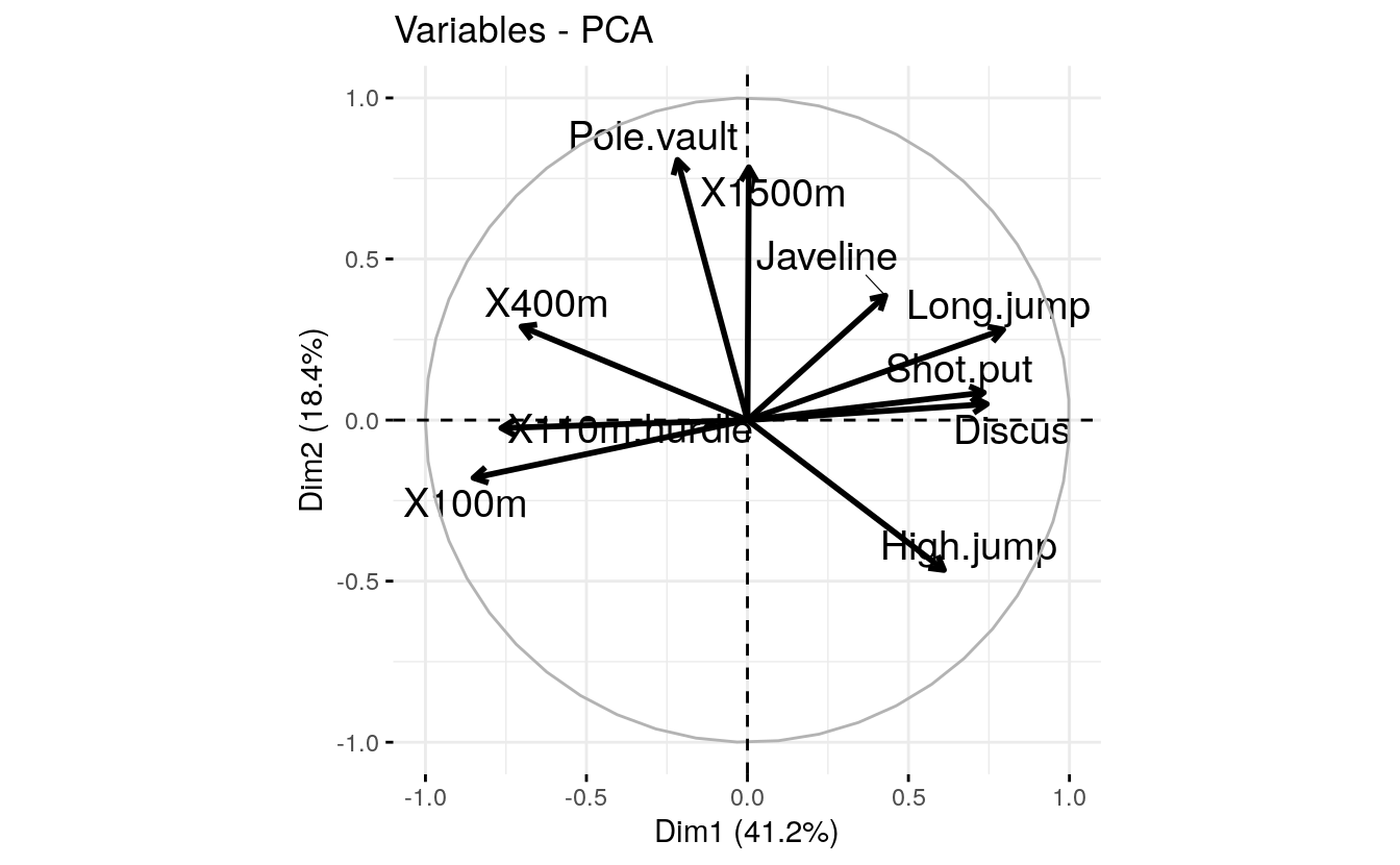

4.16 Ellipses

# Add confidence ellipses
fviz_pca_ind(iris.pca, geom.ind = "point", 
             col.ind = iris$Species, # color by groups
             palette = c("#00AFBB", "#E7B800", "#FC4E07"),
             addEllipses = TRUE, ellipse.type = "confidence",
             legend.title = "Groups"
             )
# Convex hull
fviz_pca_ind(iris.pca, geom.ind = "point",
             col.ind = iris$Species, # color by groups
             palette = c("#00AFBB", "#E7B800", "#FC4E07"),
             addEllipses = TRUE, ellipse.type = "convex",
             legend.title = "Groups"
             )

4.17 Group mean points

When coloring individuals by groups (section (???)(color-ind-by-groups)), the mean points of groups (barycenters) are also displayed by default.

To remove the mean points, use the argument mean.point = FALSE.

fviz_pca_ind(iris.pca,
             geom.ind = "point", # show points only (but not "text")
             group.ind = iris$Species, # color by groups
             legend.title = "Groups",
             mean.point = FALSE)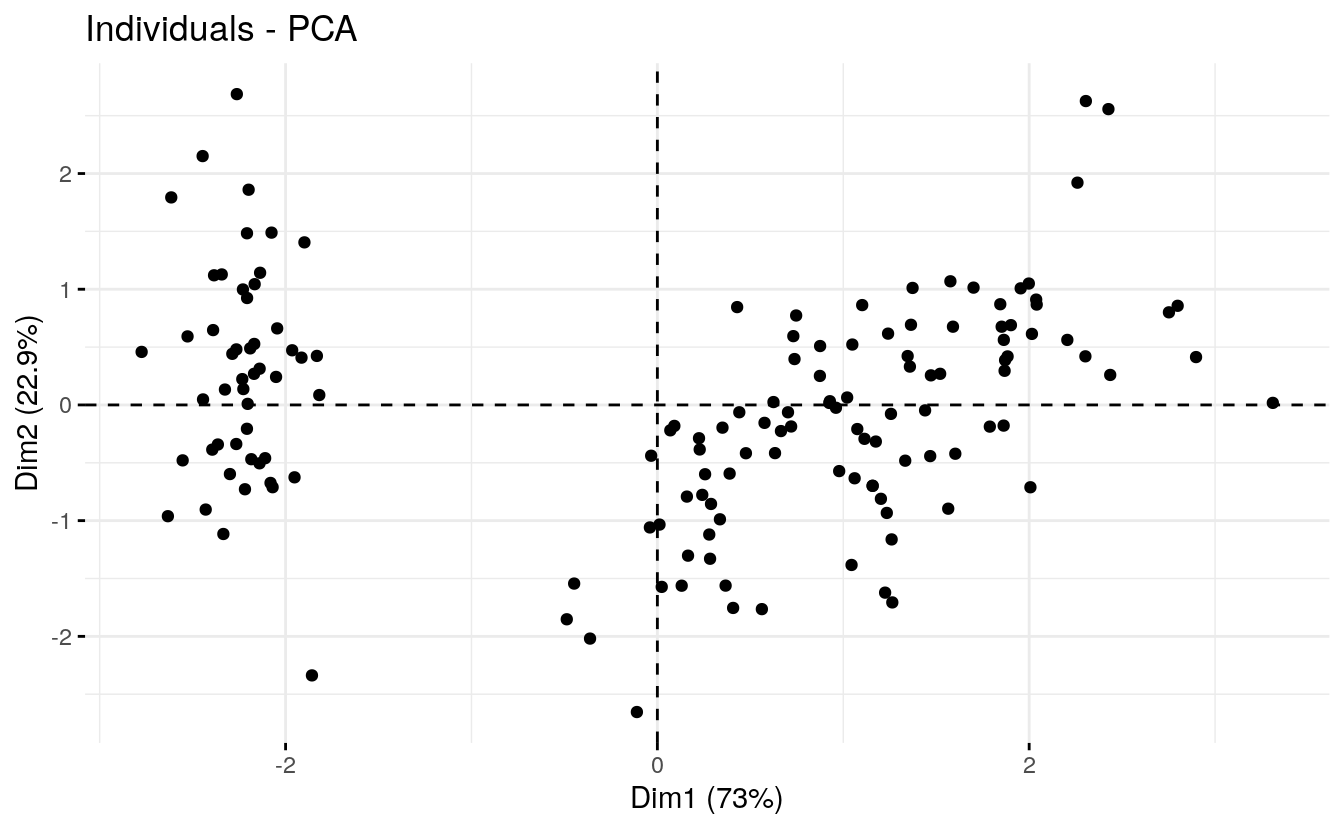

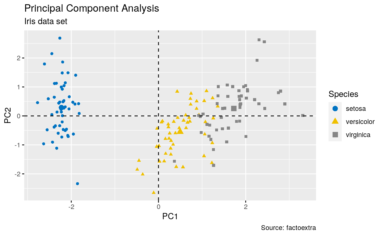
4.18 Axis lines

fviz_pca_var(res.pca, axes.linetype = "blank")

4.19 Graphical parameters

To change easily the graphical of any ggplots, you can use the function ggpar() [ggpubr package]

ind.p <- fviz_pca_ind(iris.pca, geom = "point", col.ind = iris$Species)
ggpubr::ggpar(ind.p,
              title = "Principal Component Analysis",
              subtitle = "Iris data set",
              caption = "Source: factoextra",
              xlab = "PC1", ylab = "PC2",
              legend.title = "Species", legend.position = "top",
              ggtheme = theme_gray(), palette = "jco"
              )

4.20 Biplot

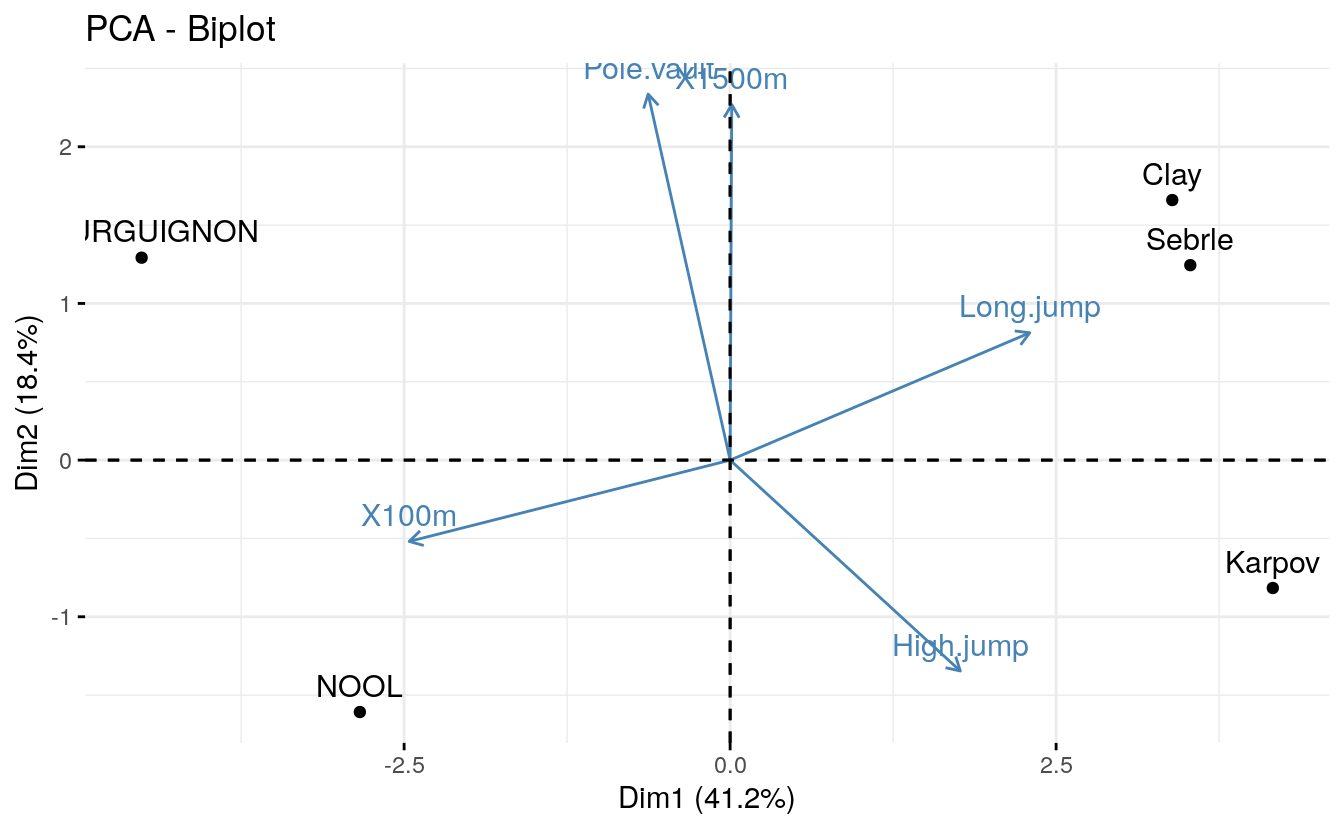
To make a simple biplot of individuals and variables, type this:

fviz_pca_biplot(res.pca, repel = TRUE,
                col.var = "#2E9FDF", # Variables color
                col.ind = "#696969"  # Individuals color
                )

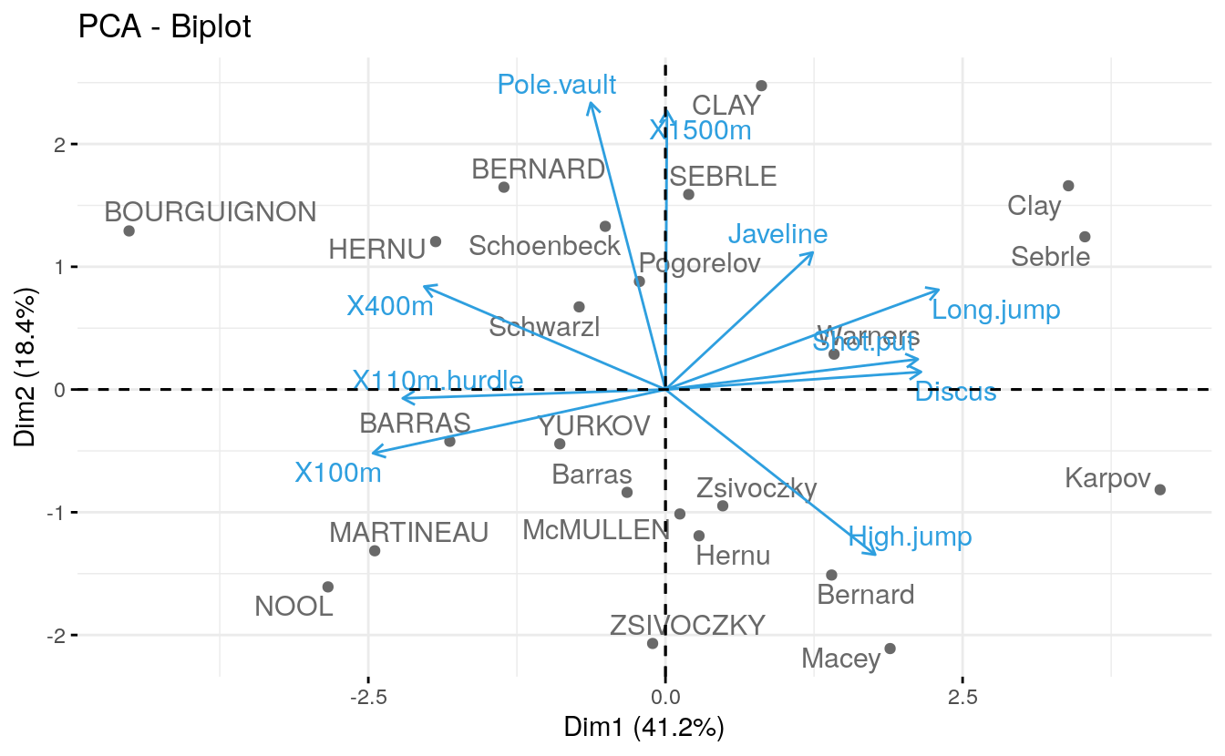
Note that, the biplot might be only useful when there is a low number of variables and individuals in the data set; otherwise the final plot would be unreadable.

Note also that, the coordinate of individuals and variables are not constructed on the same space. Therefore, in the biplot, you should mainly focus on the direction of variables but not on their absolute positions on the plot.

Roughly speaking a biplot can be interpreted as follow: * an individual that is on the same side of a given variable has a high value for this variable; * an individual that is on the opposite side of a given variable has a low value for this variable.

fviz_pca_biplot(iris.pca, 
                col.ind = iris$Species, palette = "jco", 
                addEllipses = TRUE, label = "var",
                col.var = "black", repel = TRUE,
                legend.title = "Species")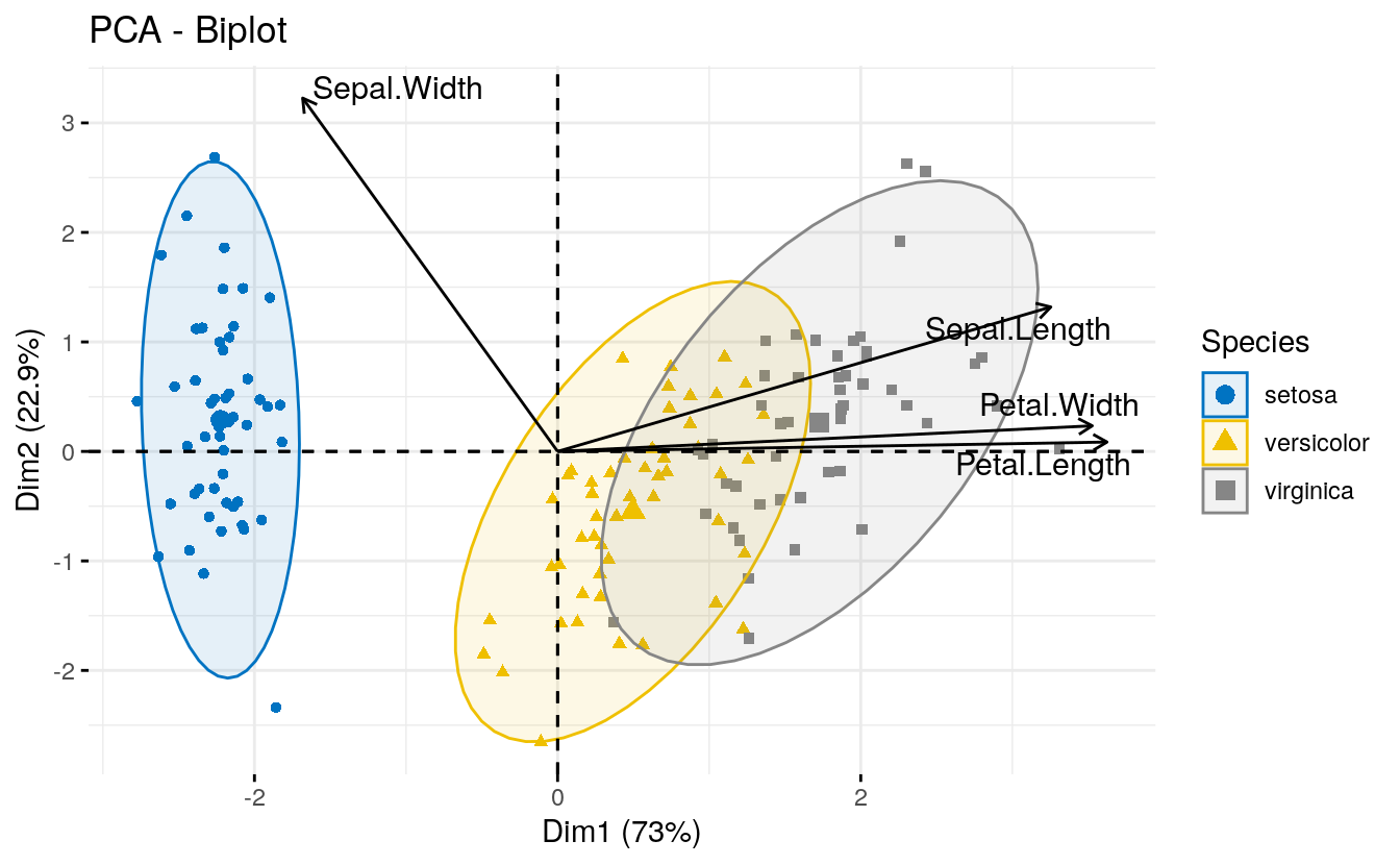 

In the following example, we want to color both individuals and variables by groups. The trick is to use pointshape = 21 for individual points. This particular point shape can be filled by a color using the argument fill.ind. The border line color of individual points is set to “black” using col.ind. To color variable by groups, the argument col.var will be used.

To customize individuals and variable colors, we use the helper functions fill_palette() and color_palette() [in ggpubr package].

fviz_pca_biplot(iris.pca, 
                # Fill individuals by groups
                geom.ind = "point",
                pointshape = 21,
                pointsize = 2.5,
                fill.ind = iris$Species,
                col.ind = "black",
                # Color variable by groups
                col.var = factor(c("sepal", "sepal", "petal", "petal")),
                
                legend.title = list(fill = "Species", color = "Clusters"),
                repel = TRUE        # Avoid label overplotting
             )+
  ggpubr::fill_palette("jco")+      # Indiviual fill color
  ggpubr::color_palette("npg")      # Variable colors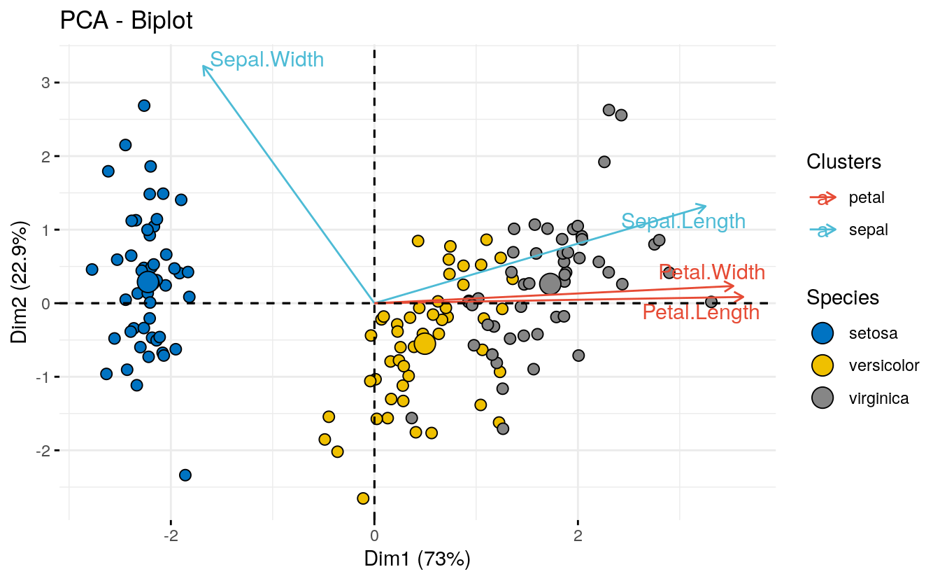

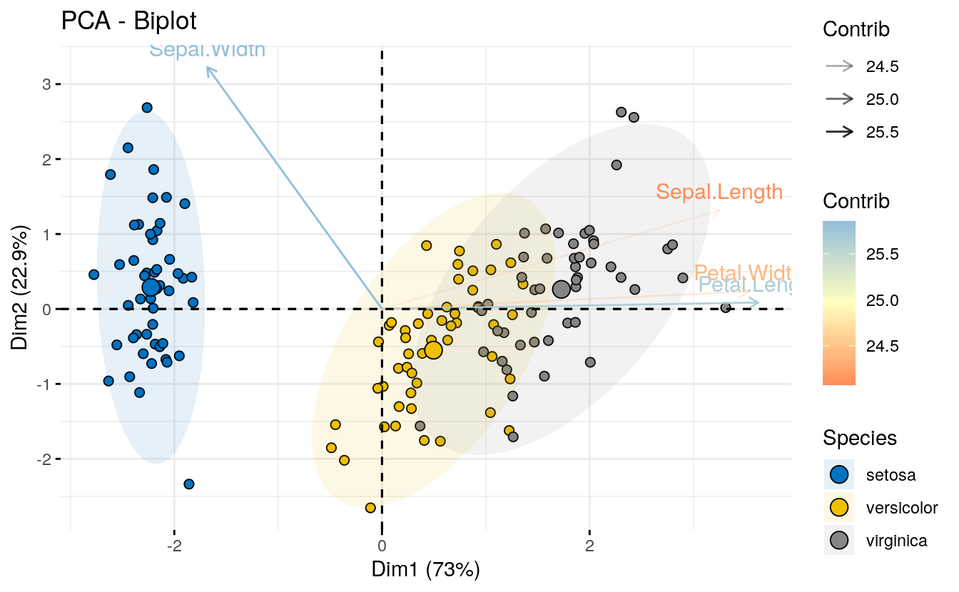
Another complex example is to color individuals by groups (discrete color) and variables by their contributions to the principal components (gradient colors). Additionally, we’ll change the transparency of variables by their contributions using the argument alpha.var.

fviz_pca_biplot(iris.pca, 
                # Individuals
                geom.ind = "point",
                fill.ind = iris$Species, col.ind = "black",
                pointshape = 21, pointsize = 2,
                palette = "jco",
                addEllipses = TRUE,
                # Variables
                alpha.var ="contrib", col.var = "contrib",
                gradient.cols = "RdYlBu",
                
                legend.title = list(fill = "Species", color = "Contrib",
                                    alpha = "Contrib")
                )

4.21 Supplementary elements

Definition and types As described above (section (???)(pca-data-format)), the decathlon2 datasets contain supplementary continuous variables (quanti.sup, columns 11:12), supplementary qualitative variables (quali.sup, column 13) and supplementary individuals (ind.sup, rows 24:27).

Supplementary variables and individuals are not used for the determination of the principal components. Their coordinates are predicted using only the information provided by the performed principal component analysis on active variables/individuals.

Specification in PCA To specify supplementary individuals and variables, the function PCA() can be used as follow:

res.pca <- PCA(decathlon2, ind.sup = 24:27, 
               quanti.sup = 11:12, quali.sup = 13, graph=FALSE)

4.22 Quantitative variables

Predicted results (coordinates, correlation and cos2) for the supplementary quantitative variables:

res.pca$quanti.sup
#> $coord
#>         Dim.1   Dim.2  Dim.3   Dim.4   Dim.5
#> Rank   -0.701 -0.2452 -0.183  0.0558 -0.0738
#> Points  0.964  0.0777  0.158 -0.1662 -0.0311
#> 
#> $cor
#>         Dim.1   Dim.2  Dim.3   Dim.4   Dim.5
#> Rank   -0.701 -0.2452 -0.183  0.0558 -0.0738
#> Points  0.964  0.0777  0.158 -0.1662 -0.0311
#> 
#> $cos2
#>        Dim.1   Dim.2  Dim.3   Dim.4   Dim.5
#> Rank   0.492 0.06012 0.0336 0.00311 0.00545
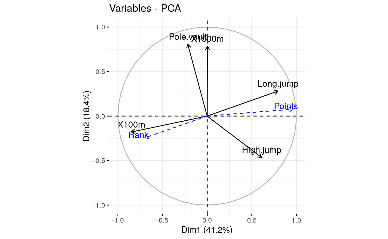
#> Points 0.929 0.00603 0.0250 0.02763 0.00097

Visualize all variables (active and supplementary ones):

fviz_pca_var(res.pca)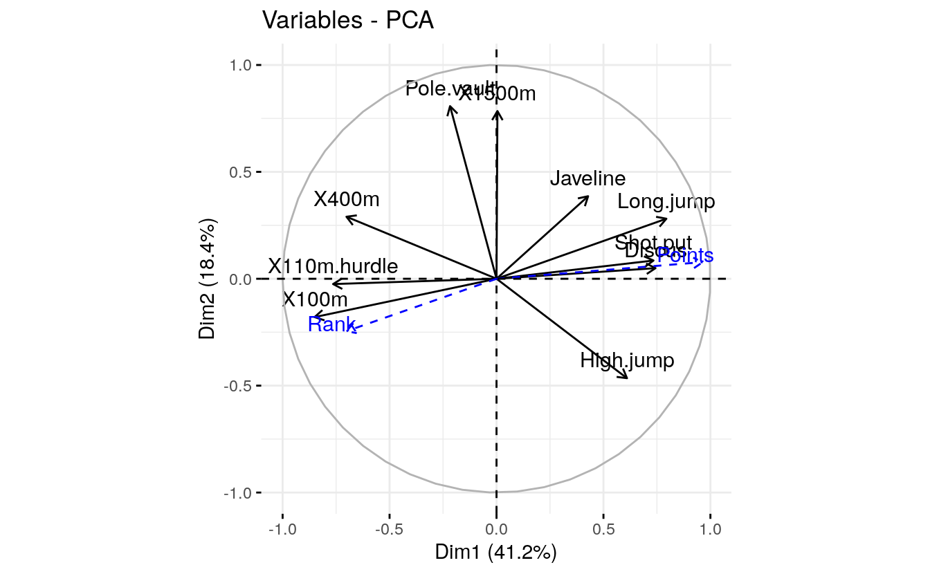

Note that, by default, supplementary quantitative variables are shown in blue color and dashed lines.

Further arguments to customize the plot:

# Change color of variables
fviz_pca_var(res.pca,
             col.var = "black",     # Active variables
             col.quanti.sup = "red" # Suppl. quantitative variables
             )
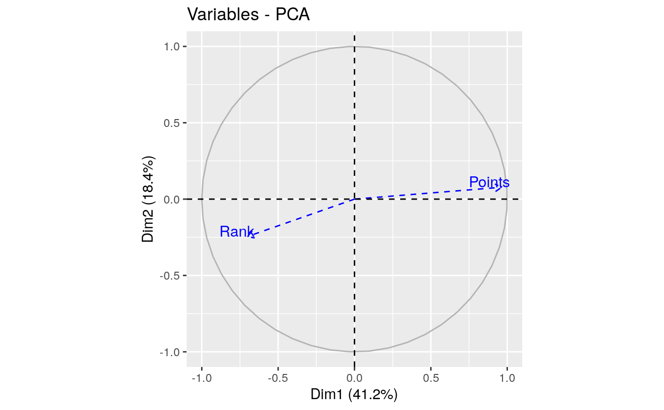
# Hide active variables on the plot, 
# show only supplementary variables
fviz_pca_var(res.pca, invisible = "var")
# Hide supplementary variables
fviz_pca_var(res.pca, invisible = "quanti.sup")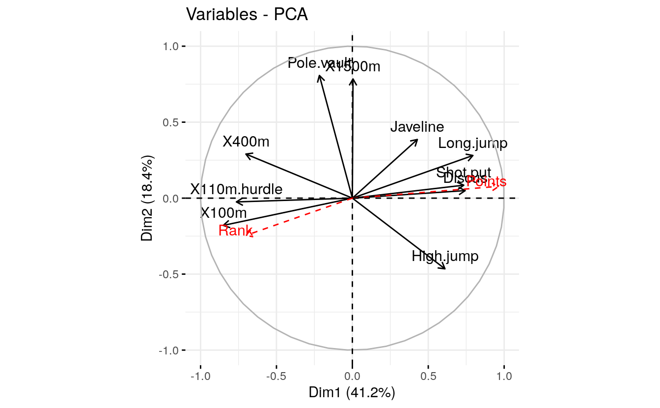

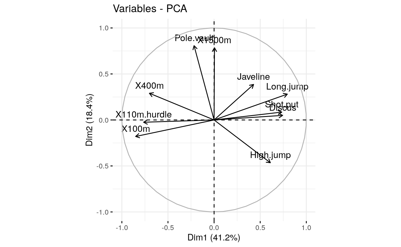
Using the fviz_pca_var(), the quantitative supplementary variables are displayed automatically on the correlation circle plot. Note that, you can add the quanti.sup variables manually, using the fviz_add() function, for further customization. An example is shown below.

# Plot of active variables
p <- fviz_pca_var(res.pca, invisible = "quanti.sup")
# Add supplementary active variables
fviz_add(p, res.pca$quanti.sup$coord, 
         geom = c("arrow", "text"), 
         color = "red")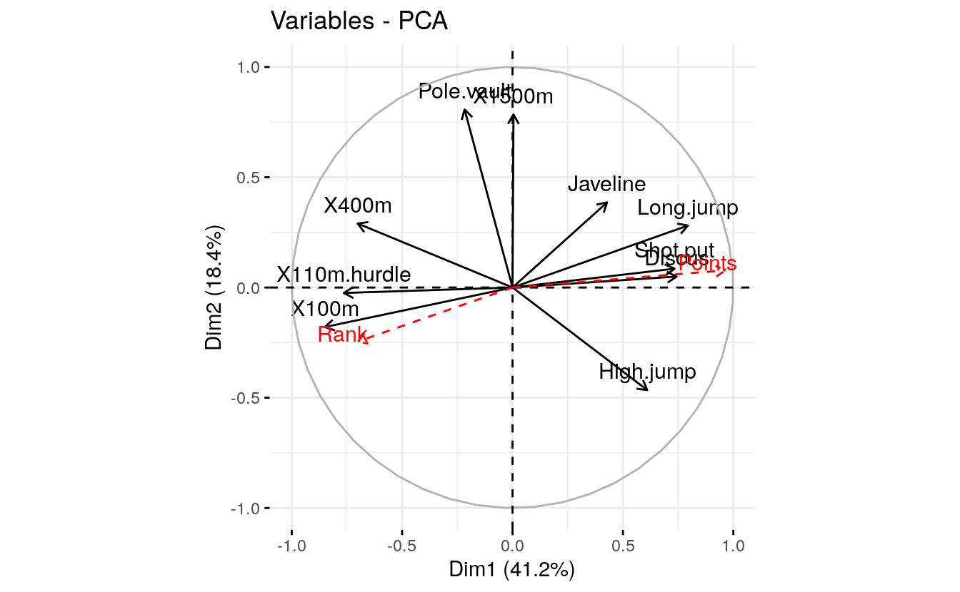

4.23 Individuals

Predicted results for the supplementary individuals (ind.sup):

res.pca$ind.sup
#> $coord
#>          Dim.1   Dim.2  Dim.3  Dim.4   Dim.5
#> KARPOV   0.795  0.7795 -1.633  1.724 -0.7507
#> WARNERS -0.386 -0.1216 -1.739 -0.706 -0.0323
#> Nool    -0.559  1.9775 -0.483 -2.278 -0.2546
#> Drews   -1.109  0.0174 -3.049 -1.534 -0.3264
#> 
#> $cos2
#>          Dim.1    Dim.2  Dim.3  Dim.4    Dim.5
#> KARPOV  0.0510 4.91e-02 0.2155 0.2403 0.045549
#> WARNERS 0.0242 2.40e-03 0.4904 0.0809 0.000169
#> Nool    0.0290 3.62e-01 0.0216 0.4811 0.006008
#> Drews   0.0921 2.27e-05 0.6956 0.1762 0.007974
#> 
#> $dist
#>  KARPOV WARNERS    Nool   Drews 
#>    3.52    2.48    3.28    3.66

Visualize all individuals (active and supplementary ones). On the graph, you can add also the supplementary qualitative variables (quali.sup), which coordinates is accessible using res.pca\(quali.supp\)coord.

p <- fviz_pca_ind(res.pca, col.ind.sup = "blue", repel = TRUE)
p <- fviz_add(p, res.pca$quali.sup$coord, color = "red")
p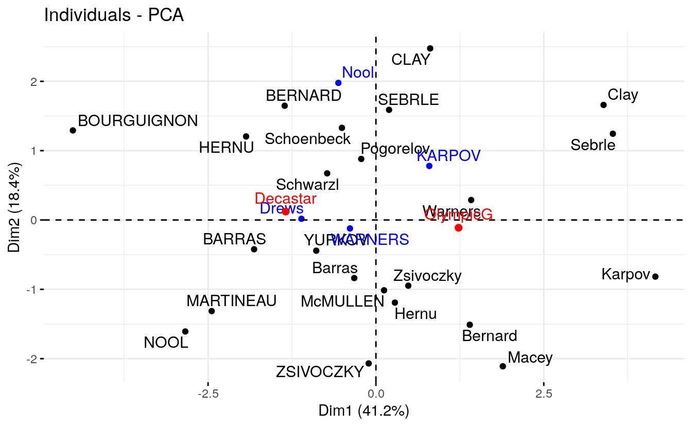

Supplementary individuals are shown in blue. The levels of the supplementary qualitative variable are shown in red color.

4.24 Qualitative variables

In the previous section, we showed that you can add the supplementary qualitative variables on individuals plot using fviz_add().

Note that, the supplementary qualitative variables can be also used for coloring individuals by groups. This can help to interpret the data. The data sets decathlon2 contain a supplementary qualitative variable at columns 13 corresponding to the type of competitions.

The results concerning the supplementary qualitative variable are:

res.pca$quali
#> $coord
#>          Dim.1  Dim.2   Dim.3  Dim.4  Dim.5
#> Decastar -1.34  0.122 -0.0379  0.181  0.134
#> OlympicG  1.23 -0.112  0.0347 -0.166 -0.123
#> 
#> $cos2
#>          Dim.1   Dim.2   Dim.3  Dim.4   Dim.5
#> Decastar 0.905 0.00744 0.00072 0.0164 0.00905
#> OlympicG 0.905 0.00744 0.00072 0.0164 0.00905
#> 
#> $v.test
#>          Dim.1  Dim.2  Dim.3  Dim.4 Dim.5
#> Decastar -2.97  0.403 -0.153  0.897  0.72
#> OlympicG  2.97 -0.403  0.153 -0.897 -0.72
#> 
#> $dist
#> Decastar OlympicG 
#>     1.41     1.29 
#> 
#> $eta2
#>             Dim.1  Dim.2   Dim.3  Dim.4  Dim.5
#> Competition 0.401 0.0074 0.00106 0.0366 0.0236

To color individuals by a supplementary qualitative variable, the argument habillage is used to specify the index of the supplementary qualitative variable. Historically, this argument name comes from the FactoMineR package. It’s a french word meaning “dressing” in english. To keep consistency between FactoMineR and factoextra, we decided to keep the same argument name

fviz_pca_ind(res.pca, habillage = 13,
             addEllipses =TRUE, ellipse.type = "confidence",
             palette = "jco", repel = TRUE)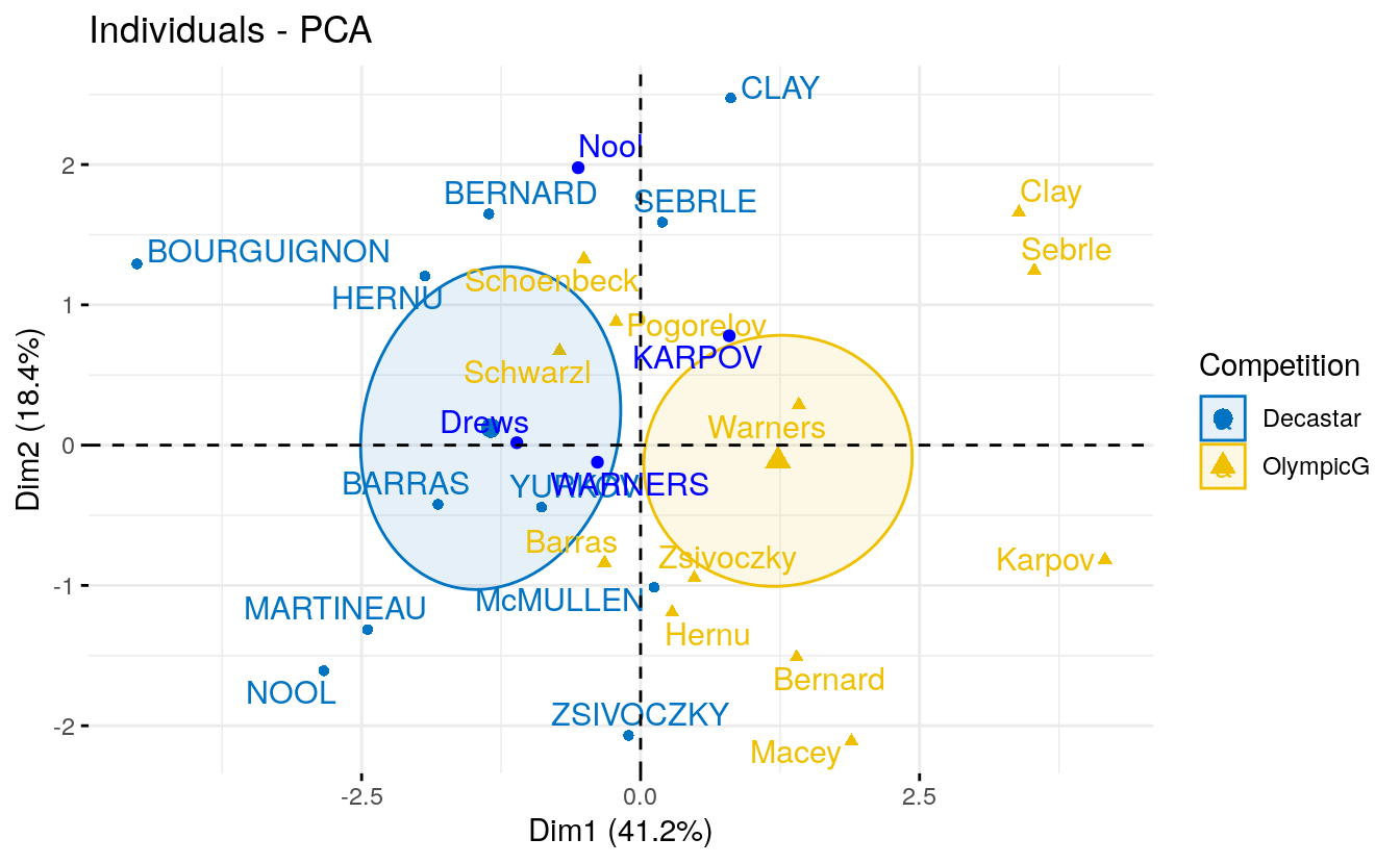 

Recall that, to remove the mean points of groups, specify the argument mean.point = FALSE.

4.25 Filtering results

If you have many individuals/variable, it’s possible to visualize only some of them using the arguments select.ind and select.var.

# Visualize variable with cos2 >= 0.6
fviz_pca_var(res.pca, select.var = list(cos2 = 0.6))
# Top 5 active variables with the highest cos2
fviz_pca_var(res.pca, select.var= list(cos2 = 5))
# Select by names
name <- list(name = c("Long.jump", "High.jump", "X100m"))
fviz_pca_var(res.pca, select.var = name)
# top 5 contributing individuals and variable
fviz_pca_biplot(res.pca, select.ind = list(contrib = 5), 
               select.var = list(contrib = 5),
               ggtheme = theme_minimal())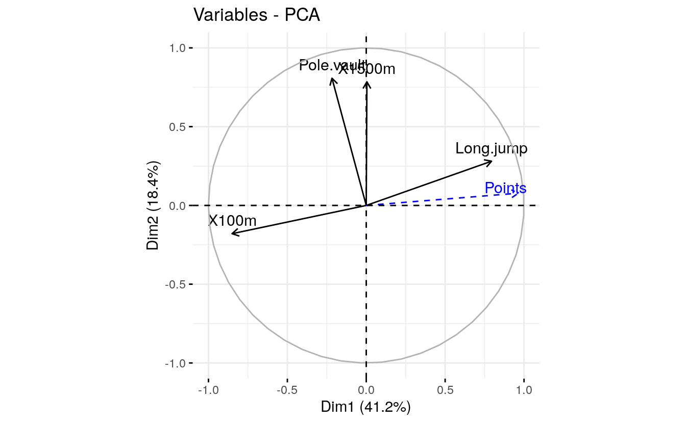

When the selection is done according to the contribution values, supplementary individuals/variables are not shown because they don’t contribute to the construction of the axes.

4.26 Exporting results

Export plots to PDF/PNG files The factoextra package produces a ggplot2-based graphs. To save any ggplots, the standard R code is as follow:

# Print the plot to a pdf file
pdf("myplot.pdf")
print(myplot)
dev.off()

In the following examples, we’ll show you how to save the different graphs into pdf or png files.

The first step is to create the plots you want as an R object:

# Scree plot
scree.plot <- fviz_eig(res.pca)
# Plot of individuals
ind.plot <- fviz_pca_ind(res.pca)
# Plot of variables
var.plot <- fviz_pca_var(res.pca)

pdf(file.path(data_out_dir, "PCA.pdf"))   # Create a new pdf device
print(scree.plot)
print(ind.plot)
print(var.plot)
dev.off() # Close the pdf device
#> png 
#>   2

Note that, using the above R code will create the PDF file into your current working directory. To see the path of your current working directory, type getwd() in the R console.

To print each plot to specific png file, the R code looks like this:

# Print scree plot to a png file
png(file.path(data_out_dir, "pca-scree-plot.png"))
print(scree.plot)
dev.off()
#> png 
#>   2
# Print individuals plot to a png file
png(file.path(data_out_dir, "pca-variables.png"))
print(var.plot)
dev.off()
#> png 
#>   2
# Print variables plot to a png file
png(file.path(data_out_dir, "pca-individuals.png"))
print(ind.plot)
dev.off()
#> png 
#>   2

Another alternative, to export ggplots, is to use the function ggexport() [in ggpubr package]. We like ggexport(), because it’s very simple. With one line R code, it allows us to export individual plots to a file (pdf, eps or png) (one plot per page). It can also arrange the plots (2 plot per page, for example) before exporting them. The examples below demonstrates how to export ggplots using ggexport().

Export individual plots to a pdf file (one plot per page):

library(ggpubr)
#> Loading required package: magrittr
ggexport(plotlist = list(scree.plot, ind.plot, var.plot), 
         filename = file.path(data_out_dir, "PCA.pdf"))
#> file saved to ../output/data/PCA.pdf

Arrange and export. Specify nrow and ncol to display multiple plots on the same page:

ggexport(plotlist = list(scree.plot, ind.plot, var.plot), 
         nrow = 2, ncol = 2,
         filename = file.path(data_out_dir, "PCA.pdf"))
#> file saved to ../output/data/PCA.pdf

Export plots to png files. If you specify a list of plots, then multiple png files will be automatically created to hold each plot.

ggexport(plotlist = list(scree.plot, ind.plot, var.plot),
         filename = file.path(data_out_dir, "PCA.png"))
#> [1] "../output/data/PCA%03d.png"
#> file saved to ../output/data/PCA%03d.png

4.27 Export results to txt/csv files

All the outputs of the PCA (individuals/variables coordinates, contributions, etc) can be exported at once, into a TXT/CSV file, using the function write.infile() [in FactoMineR] package:

# Export into a TXT file
write.infile(res.pca, file.path(data_out_dir, "pca.txt"), sep = "\t")
# Export into a CSV file
write.infile(res.pca, file.path(data_out_dir, "pca.csv"), sep = ";")

4.28 Summary

In conclusion, we described how to perform and interpret principal component analysis (PCA). We computed PCA using the PCA() function [FactoMineR]. Next, we used the factoextra R package to produce ggplot2-based visualization of the PCA results.

There are other functions [packages] to compute PCA in R:

1. Using prcomp() [stats]

res.pca <- prcomp(iris[, -5], scale. = TRUE)

res.pca <- princomp(iris[, -5], cor = TRUE)

3. Using dudi.pca() [ade4]

library(ade4)
#> 
#> Attaching package: 'ade4'
#> The following object is masked from 'package:FactoMineR':
#> 
#>     reconst
res.pca <- dudi.pca(iris[, -5], scannf = FALSE, nf = 5)

4. Using epPCA() [ExPosition]

library(ExPosition)
#> Loading required package: prettyGraphs
res.pca <- epPCA(iris[, -5], graph = FALSE)

No matter what functions you decide to use, in the list above, the factoextra package can handle the output for creating beautiful plots similar to what we described in the previous sections for FactoMineR:

fviz_eig(res.pca)     # Scree plot
fviz_pca_ind(res.pca) # Graph of individuals
fviz_pca_var(res.pca) # Graph of variables