30 Prediction of arrhythmia with deep neural nets
30.1 Introduction
27 February 2017
This week, I am showing how to build feed-forward deep neural networks or multilayer perceptrons. The models in this example are built to classify ECG data into being either from healthy hearts or from someone suffering from arrhythmia. I will show how to prepare a dataset for modeling, setting weights and other modeling parameters, and finally, how to evaluate model performance with the h2o package.
30.1.1 Deep learning with neural networks
Deep learning with neural networks is arguably one of the most rapidly growing applications of machine learning and AI today. They allow building complex models that consist of multiple hidden layers within artificial networks and are able to find non-linear patterns in unstructured data. Deep neural networks are usually feed-forward, which means that each layer feeds its output to subsequent layers, but recurrent or feed-back neural networks can also be built. Feed-forward neural networks are also called multilayer perceptrons (MLPs).
30.1.2 H2O
The R package h2o provides a convenient interface to H2O, which is an open-source machine learning and deep learning platform. H2O distributes a wide range of common machine learning algorithms for classification, regression and deep learning.
30.1.3 Preparing the R session
First, we need to load the packages.
library(dplyr)
library(h2o)
library(ggplot2)
library(ggrepel)
library(h2o)

h2o.init()
#>  Connection successful!
#>
#> R is connected to the H2O cluster:
#>     H2O cluster uptime:         26 minutes 32 seconds
#>     H2O cluster timezone:       Etc/UTC
#>     H2O data parsing timezone:  UTC
#>     H2O cluster version:        3.30.0.1
#>     H2O cluster version age:    7 months and 16 days !!!
#>     H2O cluster name:           H2O_started_from_R_root_mwl453
#>     H2O cluster total nodes:    1
#>     H2O cluster total memory:   7.23 GB
#>     H2O cluster total cores:    8
#>     H2O cluster allowed cores:  8
#>     H2O cluster healthy:        TRUE
#>     H2O Connection ip:          localhost
#>     H2O Connection port:        54321
#>     H2O Connection proxy:       NA
#>     H2O Internal Security:      FALSE
#>     H2O API Extensions:         Amazon S3, XGBoost, Algos, AutoML, Core V3, TargetEncoder, Core V4
#>     R Version:                  R version 3.6.3 (2020-02-29)
#> Warning in h2o.clusterInfo():
#> Your H2O cluster version is too old (7 months and 16 days)!
#> Please download and install the latest version from http://h2o.ai/download/
my_theme <- function(base_size = 12, base_family = "sans"){
  theme_minimal(base_size = base_size, base_family = base_family) +
  theme(
    axis.text = element_text(size = 12),
    axis.title = element_text(size = 14),
    panel.grid.major = element_line(color = "grey"),
    panel.grid.minor = element_blank(),
    panel.background = element_rect(fill = "aliceblue"),
    strip.background = element_rect(fill = "darkgrey", color = "grey", size = 1),
    strip.text = element_text(face = "bold", size = 12, color = "white"),
    legend.position = "right",
    legend.justification = "top",
    panel.border = element_rect(color = "grey", fill = NA, size = 0.5)
  )
}
30.2 Arrhythmia data
The data I am using to demonstrate the building of neural nets is the arrhythmia dataset from UC Irvine’s machine learning database. It contains 279 features from ECG heart rhythm diagnostics and one output column. I am not going to rename the feature columns because they are too many and the descriptions are too complex. Also, we don’t need to know specifically which features we are looking at for building the models.
For a description of each feature, see https://archive.ics.uci.edu/ml/machine-learning-databases/arrhythmia/arrhythmia.names.
The output column defines 16 classes: class 1 samples are from healthy ECGs, the remaining classes belong to different types of arrhythmia, with class 16 being all remaining arrhythmia cases that didn’t fit into distinct classes.
arrhythmia <- read.table(file.path(data_raw_dir, "arrhythmia.data.txt"), sep = ",")
arrhythmia[arrhythmia == "?"] <- NA

# making sure, that all feature columns are numeric
arrhythmia[-280] <- lapply(arrhythmia[-280], as.character)
arrhythmia[-280] <- lapply(arrhythmia[-280], as.numeric)

#  renaming output column and converting to factor
colnames(arrhythmia)[280] <- "class"
arrhythmia$class <- as.factor(arrhythmia$class)
As usual, I want to get acquainted with the data and explore it’s properties before I am building any model. So, I am first going to look at the distribution of classes and of healthy and arrhythmia samples.
Because I am interested in distinguishing healthy from arrhythmia ECGs, I am converting the output to binary format by combining all arrhythmia cases into one class.
#  all arrhythmia cases into one class
arrhythmia$diagnosis <- ifelse(arrhythmia$class == 1, "healthy", "arrhythmia")
arrhythmia$diagnosis <- as.factor(arrhythmia$diagnosis)
library(gridExtra)
#>
#> Attaching package: 'gridExtra'
#> The following object is masked from 'package:dplyr':
#>
#>     combine
library(grid)

grid.arrange(p1, p2, ncol = 2)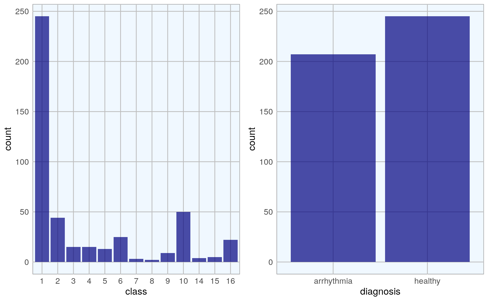
With binary classification, we have almost the same numbers of healthy and arrhythmia cases in our dataset.
I am also interested in how much the normal and arrhythmia cases cluster in a Principal Component Analysis (PCA). I am first preparing the PCA plotting function and then run it on the feature data.
library(pcaGoPromoter)

pca_func <- function(pcaOutput2, group_name){
    centroids <- aggregate(cbind(PC1, PC2) ~ groups, pcaOutput2, mean)
    conf.rgn  <- do.call(rbind, lapply(unique(pcaOutput2$groups), function(t)
          data.frame(groups = as.character(t),
                     ellipse(cov(pcaOutput2[pcaOutput2$groups == t, 1:2]),
                           centre = as.matrix(centroids[centroids$groups == t, 2:3]),
                           level = 0.95),
                     stringsAsFactors = FALSE)))

    plot <- ggplot(data = pcaOutput2, aes(x = PC1, y = PC2, group = groups,
                                          color = groups)) +
      geom_polygon(data = conf.rgn, aes(fill = groups), alpha = 0.2) +
      geom_point(size = 2, alpha = 0.5) +
      labs(color = paste(group_name),
           fill = paste(group_name),
           x = paste0("PC1: ", round(pcaOutput$pov[1], digits = 2) * 100, "% variance"),
           y = paste0("PC2: ", round(pcaOutput$pov[2], digits = 2) * 100, "% variance")) +
      my_theme()

    return(plot)
}
# Find what columns have NAs and the quantity
for (col in names(arrhythmia)) {
    n_nas <- length(which(is.na(arrhythmia[, col])))
    if (n_nas > 0) cat(col, n_nas, "\n")
}
#> V11 8
#> V12 22
#> V13 1
#> V14 376
#> V15 1
# Replace NAs with zeros
arrhythmia[is.na(arrhythmia)] <- 0
Find and plot the PCAs.
pcaOutput <- pca(t(arrhythmia[-c(280, 281)]), printDropped=FALSE,
                 scale=TRUE,
                 center = TRUE)

pcaOutput2 <- as.data.frame(pcaOutput$scores)

pcaOutput2$groups <- arrhythmia$class
p1 <- pca_func(pcaOutput2, group_name = "class")

pcaOutput2$groups <- arrhythmia$diagnosis
p2 <- pca_func(pcaOutput2, group_name = "diagnosis")

grid.arrange(p1, p2, ncol = 2)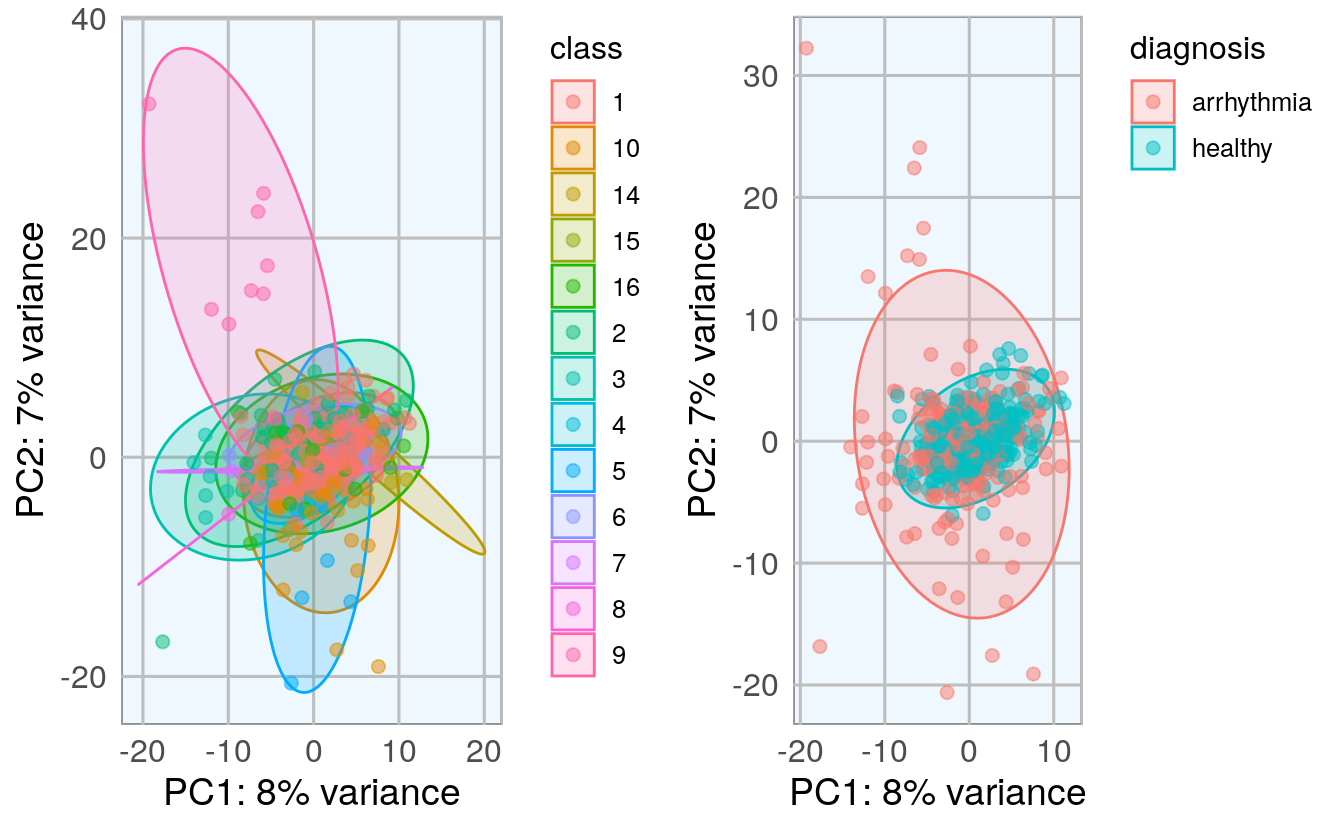
The PCA shows that there is a big overlap between healthy and arrhythmia samples, i.e. there does not seem to be major global differences in all features. The class that is most distinct from all others seems to be class 9.
I want to give the arrhythmia cases that are very different from the rest a stronger weight in the neural network, so I define a weight column where every sample outside the central PCA cluster will get a “2”, they will in effect be used twice in the model.
I also want to know what the variance is within features.
library(matrixStats)
#>
#> Attaching package: 'matrixStats'
#> The following object is masked from 'package:dplyr':
#>
#>     count

colvars <- data.frame(feature = colnames(arrhythmia[-c(280, 281)]),
                      variance = colVars(as.matrix(arrhythmia[-c(280, 281)])))

subset(colvars, variance > 50) %>%
  mutate(feature = factor(feature, levels = colnames(arrhythmia[-c(280, 281)]))) %>%
  ggplot(aes(x = feature, y = variance)) +
    geom_bar(stat = "identity", fill = "navy", alpha = 0.7) +
    my_theme() +
    theme(axis.text.x = element_text(angle = 90, vjust = 0.5, hjust = 1))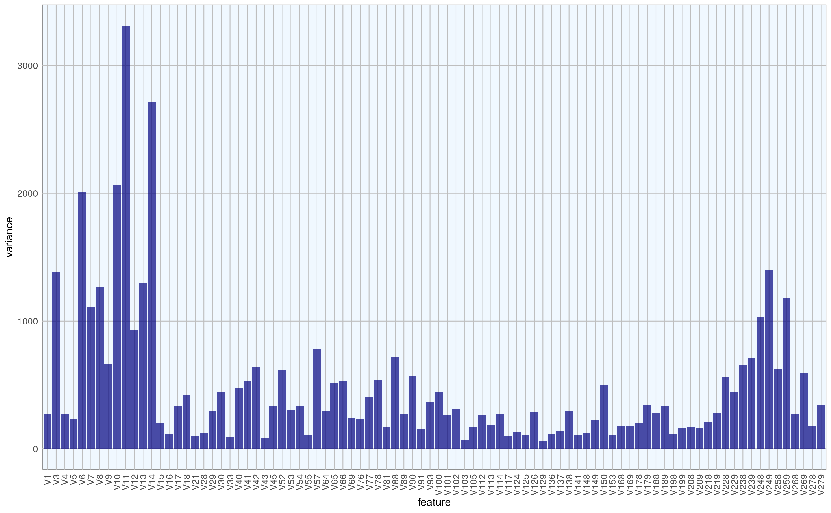
Features with low variance are less likely to strongly contribute to a differentiation between healthy and arrhythmia cases, so I am going to remove them. I am also concatenating the weights column:
30.3 Converting the dataframe to a h2o object
Now that I have my final data frame for modeling, for working with h2o functions, the data needs to be converted from a DataFrame to an H2O Frame. This is done with the as_h2o_frame() function.
#as_h2o_frame(arrhythmia_subset)
arrhythmia_hf <- as.h2o(arrhythmia_subset, key="arrhtythmia.hex")
#>
  |
  |                                                                      |   0%
  |
  |======================================================================| 100%
We can now access all functions from the h2o package that are built to work on h2o Frames. A useful such function is h2o.describe(). It is similar to base R’s summary() function but outputs many more descriptive measures for our data. To get a good overview about these measures, I am going to plot them.
library(tidyr) # for gathering
#>
#> Attaching package: 'tidyr'
#> The following object is masked from 'package:S4Vectors':
#>
#>     expand
h2o.describe(arrhythmia_hf[, -1]) %>% # excluding the weights column
  gather(x, y, Zeros:Sigma) %>%
  mutate(group = ifelse(
    x %in% c("Min", "Max", "Mean"), "min, mean, max",
    ifelse(x %in% c("NegInf", "PosInf"), "Inf", "sigma, zeros"))) %>%
  # separating them into facets makes them easier to see
  mutate(Label = factor(Label, levels = colnames(arrhythmia_hf[, -1]))) %>%
  ggplot(aes(x = Label, y = as.numeric(y), color = x)) +
    geom_point(size = 4, alpha = 0.6) +
    scale_color_brewer(palette = "Set1") +
    my_theme() +
    theme(axis.text.x = element_text(angle = 90, vjust = 0.5, hjust = 1)) +
    facet_grid(group ~ ., scales = "free") +
    labs(x = "Feature",
         y = "Value",
         color = "")
#> Warning: Removed 2 rows containing missing values (geom_point).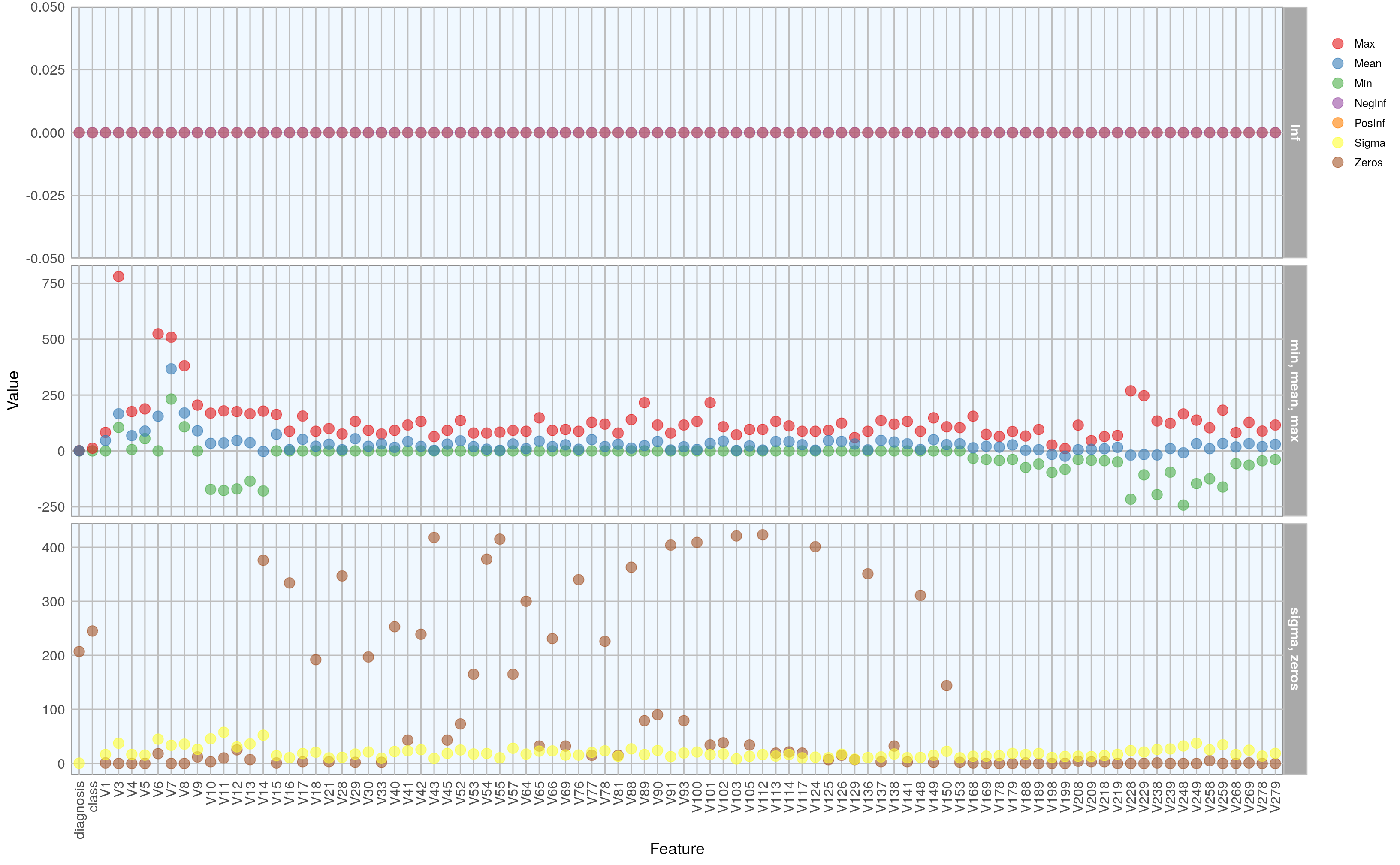
I am also interested in the correlation between features and the output. We can use the h2o.cor() function to calculate the correlation matrix. It is again much easier to understand the data when we visualize it, so I am going to create another plot.
library(reshape2) # for melting
#>
#> Attaching package: 'reshape2'
#> The following object is masked from 'package:tidyr':
#>
#>     smiths

# diagnosis is now a characer column and we need to convert it again
arrhythmia_hf[, 2] <- h2o.asfactor(arrhythmia_hf[, 2])
arrhythmia_hf[, 3] <- h2o.asfactor(arrhythmia_hf[, 3]) # same for class

cor <- h2o.cor(arrhythmia_hf[, -c(1, 3)])
rownames(cor) <- colnames(cor)

melt(cor) %>%
  mutate(Var2 = rep(rownames(cor), nrow(cor))) %>%
  mutate(Var2 = factor(Var2, levels = colnames(cor))) %>%
  mutate(variable = factor(variable, levels = colnames(cor))) %>%
  ggplot(aes(x = variable, y = Var2, fill = value)) +
    geom_tile(width = 0.9, height = 0.9) +
    scale_fill_gradient2(low = "white", high = "red", name = "Cor.") +
    my_theme() +
    theme(axis.text.x = element_text(angle = 90, vjust = 0.5, hjust = 1)) +
    labs(x = "",
         y = "")
#> No id variables; using all as measure variables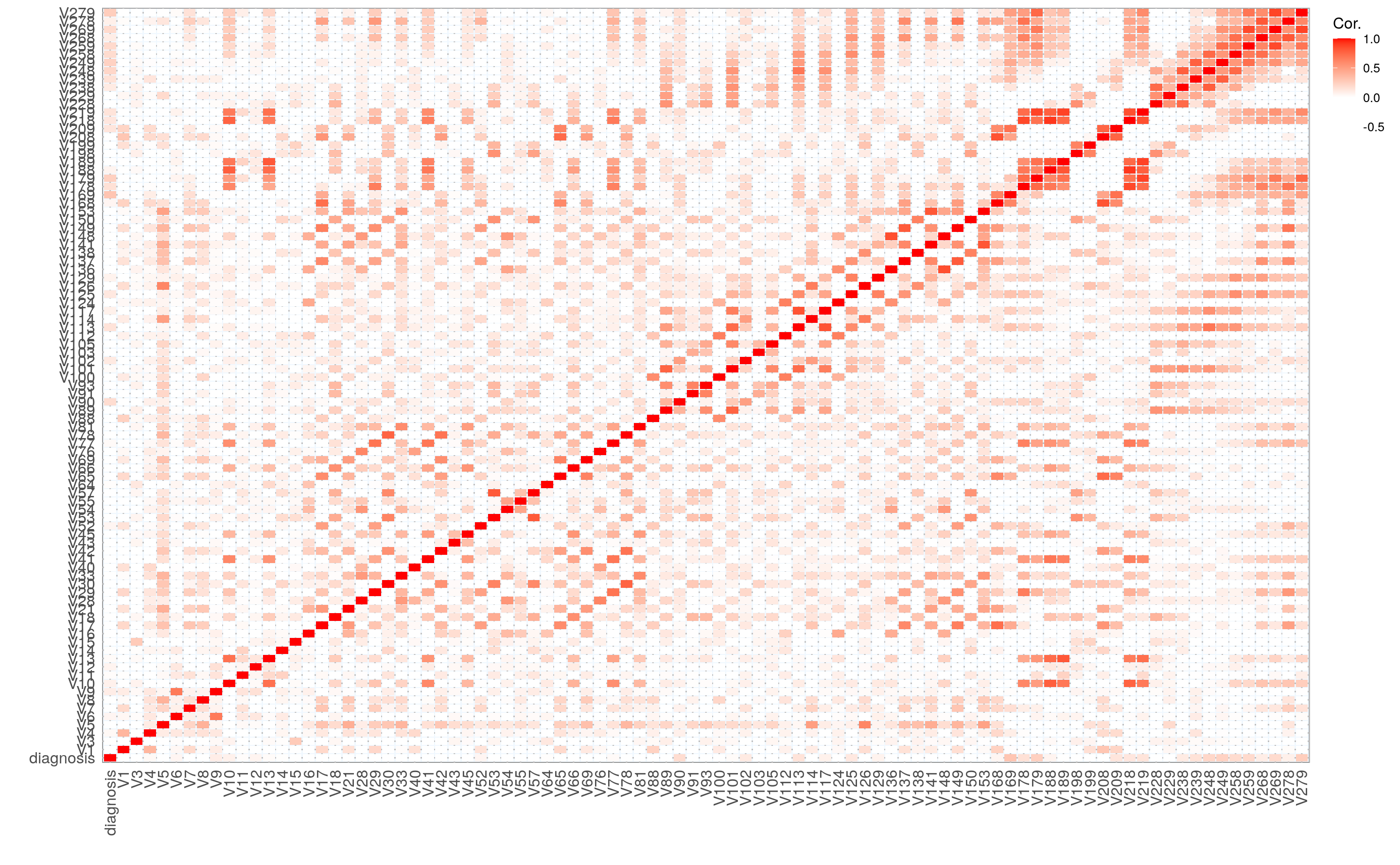
30.4 Training, test and validation data
Now we can use the h2o.splitFrame() function to split the data into training, validation and test data.
Here, I am using 70% for training and 15% each for validation and testing. We could also just split the data into two sections, a training and test set but when we have sufficient samples, it is a good idea to evaluate model performance on an independent test set on top of training with a validation set. Because we can easily overfit a model, we want to get an idea about how generalizable it is - this we can only assess by looking at how well it works on previously unknown data.
I am also defining response, features and weights column names now.
splits <- h2o.splitFrame(arrhythmia_hf,
                         ratios = c(0.7, 0.15),
                         seed = 1)

train <- splits[[1]]
valid <- splits[[2]]
test <- splits[[3]]

response <- "diagnosis"
weights <- "weights"
features <- setdiff(colnames(train), c(response, weights, "class"))
summary(train$diagnosis, exact_quantiles = TRUE)
#>  diagnosis
#>  healthy   :163
#>  arrhythmia:155
summary(valid$diagnosis, exact_quantiles = TRUE)
#>  diagnosis
#>  healthy   :43
#>  arrhythmia:25
summary(test$diagnosis, exact_quantiles = TRUE)
#>  diagnosis
#>  healthy   :39
#>  arrhythmia:27
If we had more categorical features, we could use the h2o.interaction() function to define interaction terms, but since we only have numeric features here, we don’t need this.
We can also run a PCA on the training data, using the h2o.prcomp() function to calculate the singular value decomposition of the Gram matrix with the power method.
pca <- h2o.prcomp(training_frame = train,
           x = features,
           validation_frame = valid,
           transform = "NORMALIZE",
           k = 3,
           seed = 42)
#>
  |
  |                                                                      |   0%
  |
  |==============                                                        |  20%
  |
  |======================================================================| 100%
#> Warning in doTryCatch(return(expr), name, parentenv, handler): _train: Dataset
#> used may contain fewer number of rows due to removal of rows with NA/missing
#> values. If this is not desirable, set impute_missing argument in pca call to
#> TRUE/True/true/... depending on the client language.
pca
#> Model Details:
#> ==============
#>
#> H2ODimReductionModel: pca
#> Model ID:  PCA_model_R_1605830707207_2732
#> Importance of components:
#>                             pc1      pc2      pc3
#> Standard deviation     0.582620 0.507796 0.421869
#> Proportion of Variance 0.164697 0.125110 0.086351
#> Cumulative Proportion  0.164697 0.289808 0.376159
#>
#>
#> H2ODimReductionMetrics: pca
#>
#> No model metrics available for PCA
#> H2ODimReductionMetrics: pca
#>
#> No model metrics available for PCA
eigenvec <- as.data.frame(pca@model$eigenvectors)
eigenvec$label <- features

ggplot(eigenvec, aes(x = pc1, y = pc2, label = label)) +
  geom_point(color = "navy", alpha = 0.7) +
  geom_text_repel() +
  my_theme()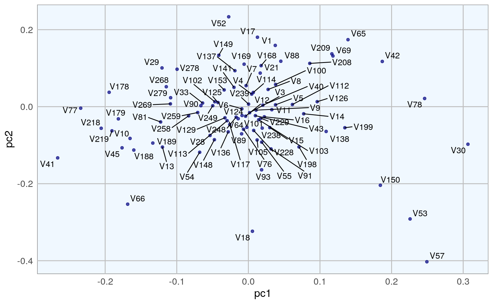
30.5 Modeling
Now, we can build a deep neural network model. We can specify quite a few parameters, like
Cross-validation: Cross validation can tell us the training and validation errors for each model. The final model will be overwritten with the best model, if we don’t specify otherwise.
Adaptive learning rate: For deep learning with h2o, we by default use stochastic gradient descent optimization with an an adaptive learning rate. The two corresponding parameters rho and epsilon help us find global (or near enough) optima.
Activation function: The activation function defines the node output relative to a given set of inputs. We want our activation function to be non-linear and continuously differentiable.
Hidden nodes: Defines the number of hidden layers and the number of nodes per layer.
Epochs: Increasing the number of epochs (one full training cycle on all training samples) can increase model performance, but we also run the risk of overfitting. To determine the optimal number of epochs, we need to use early stopping.
Early stopping: By default, early stopping is enabled. This means that training will be stopped when we reach a certain validation error to prevent overfitting.
Of course, you need quite a bit of experience and intuition to hit on a good combination of parameters. That’s why it usually makes sense to do a grid search for hyper-parameter tuning. Here, I want to focus on building and evaluating deep learning models, though. I will cover grid search in next week’s post.
# this will take some time and all CPUs
dl_model <- h2o.deeplearning(x = features,
                             y = response,
                             weights_column = weights,
                             model_id = "dl_model",
                             training_frame = train,
                             validation_frame = valid,
                             nfolds = 15,                                   # 10x cross validation
                             keep_cross_validation_fold_assignment = TRUE,
                             fold_assignment = "Stratified",
                             activation = "RectifierWithDropout",
                             score_each_iteration = TRUE,
                             hidden = c(200, 200, 200, 200, 200),           # 5 hidden layers, each of 200 neurons
                             epochs = 100,
                             variable_importances = TRUE,
                             export_weights_and_biases = TRUE,
                             seed = 42)
#>
  |
  |                                                                      |   0%
  |
  |=                                                                     |   1%
  |
  |==                                                                    |   3%
  |
  |===                                                                   |   4%
  |
  |====                                                                  |   5%
  |
  |=====                                                                 |   8%
  |
  |======                                                                |   9%
  |
  |=======                                                               |  10%
  |
  |========                                                              |  12%
  |
  |=========                                                             |  12%
  |
  |===========                                                           |  16%
  |
  |============                                                          |  17%
  |
  |==============                                                        |  19%
  |
  |==============                                                        |  21%
  |
  |================                                                      |  22%
  |
  |=================                                                     |  24%
  |
  |==================                                                    |  25%
  |
  |==================                                                    |  26%
  |
  |===================                                                   |  28%
  |
  |=====================                                                 |  30%
  |
  |======================                                                |  31%
  |
  |======================                                                |  32%
  |
  |========================                                              |  34%
  |
  |=========================                                             |  36%
  |
  |==========================                                            |  38%
  |
  |===========================                                           |  39%
  |
  |============================                                          |  40%
  |
  |=============================                                         |  41%
  |
  |==============================                                        |  42%
  |
  |====================================                                  |  51%
  |
  |=====================================                                 |  53%
  |
  |==============================================================        |  89%
  |
  |================================================================      |  92%
  |
  |=================================================================     |  92%
  |
  |==================================================================    |  94%
  |
  |===================================================================   |  96%
  |
  |====================================================================  |  97%
  |
  |====================================================================  |  98%
  |
  |===================================================================== |  99%
  |
  |======================================================================| 100%
Because training can take a while, depending on how many samples, features, nodes and hidden layers you are training on, it is a good idea to save your model.
# if file exists, overwrite it
h2o.saveModel(dl_model, path = file.path(data_out_dir, "dl_model"), force = TRUE)
#> [1] "/home/rstudio/all/output/data/dl_model/dl_model"
We can then re-load the model again any time to check the model quality and make predictions on new data.
dl_model <- h2o.loadModel(file.path(data_out_dir, "dl_model/dl_model"))30.6 Model performance
We now want to know how our model performed on the validation data. The summary() function will give us a detailed overview of our model. I am not showing the output here, because it is quite extensive.
sum_model <- summary(dl_model)
#> Model Details:
#> ==============
#>
#> H2OBinomialModel: deeplearning
#> Model Key:  dl_model
#> Status of Neuron Layers: predicting diagnosis, 2-class classification, bernoulli distribution, CrossEntropy loss, 179,402 weights/biases, 2.1 MB, 34,090 training samples, mini-batch size 1
#>   layer units             type dropout       l1       l2 mean_rate rate_rms
#> 1     1    90            Input  0.00 %       NA       NA        NA       NA
#> 2     2   200 RectifierDropout 50.00 % 0.000000 0.000000  0.004316 0.003539
#> 3     3   200 RectifierDropout 50.00 % 0.000000 0.000000  0.006148 0.003677
#> 4     4   200 RectifierDropout 50.00 % 0.000000 0.000000  0.008944 0.004507
#> 5     5   200 RectifierDropout 50.00 % 0.000000 0.000000  0.008100 0.003903
#> 6     6   200 RectifierDropout 50.00 % 0.000000 0.000000  0.021225 0.041223
#> 7     7     2          Softmax      NA 0.000000 0.000000  0.002463 0.001179
#>   momentum mean_weight weight_rms mean_bias bias_rms
#> 1       NA          NA         NA        NA       NA
#> 2 0.000000    0.003201   0.096234  0.416323 0.067160
#> 3 0.000000   -0.009090   0.074995  0.948930 0.055226
#> 4 0.000000   -0.007553   0.072301  0.964074 0.031132
#> 5 0.000000   -0.006909   0.071043  0.970670 0.031634
#> 6 0.000000   -0.009785   0.070533  0.951147 0.034766
#> 7 0.000000   -0.041089   0.377436  0.001956 0.035948
#>
#> H2OBinomialMetrics: deeplearning
#> ** Reported on training data. **
#> ** Metrics reported on full training frame **
#>
#> MSE:  0.0215
#> RMSE:  0.147
#> LogLoss:  0.0867
#> Mean Per-Class Error:  0.0214
#> AUC:  0.994
#> AUCPR:  0.993
#> Gini:  0.988
#>
#> Confusion Matrix (vertical: actual; across: predicted) for F1-optimal threshold:
#>            arrhythmia healthy    Error    Rate
#> arrhythmia        158       6 0.036585  =6/164
#> healthy             1     162 0.006135  =1/163
#> Totals            159     168 0.021407  =7/327
#>
#> Maximum Metrics: Maximum metrics at their respective thresholds
#>                         metric threshold      value idx
#> 1                       max f1  0.353389   0.978852 167
#> 2                       max f2  0.353389   0.987805 167
#> 3                 max f0point5  0.398621   0.973398 165
#> 4                 max accuracy  0.398621   0.978593 165
#> 5                max precision  0.998682   1.000000   0
#> 6                   max recall  0.019924   1.000000 175
#> 7              max specificity  0.998682   1.000000   0
#> 8             max absolute_mcc  0.353389   0.957638 167
#> 9   max min_per_class_accuracy  0.562323   0.969512 163
#> 10 max mean_per_class_accuracy  0.353389   0.978640 167
#> 11                     max tns  0.998682 164.000000   0
#> 12                     max fns  0.998682 162.000000   0
#> 13                     max fps  0.000000 164.000000 317
#> 14                     max tps  0.019924 163.000000 175
#> 15                     max tnr  0.998682   1.000000   0
#> 16                     max fnr  0.998682   0.993865   0
#> 17                     max fpr  0.000000   1.000000 317
#> 18                     max tpr  0.019924   1.000000 175
#>
#> Gains/Lift Table: Extract with `h2o.gainsLift(<model>, <data>)` or `h2o.gainsLift(<model>, valid=<T/F>, xval=<T/F>)`
#> H2OBinomialMetrics: deeplearning
#> ** Reported on validation data. **
#> ** Metrics reported on full validation frame **
#>
#> MSE:  0.18
#> RMSE:  0.424
#> LogLoss:  1.08
#> Mean Per-Class Error:  0.232
#> AUC:  0.873
#> AUCPR:  0.911
#> Gini:  0.747
#>
#> Confusion Matrix (vertical: actual; across: predicted) for F1-optimal threshold:
#>            arrhythmia healthy    Error    Rate
#> arrhythmia         14      11 0.440000  =11/25
#> healthy             1      42 0.023256   =1/43
#> Totals             15      53 0.176471  =12/68
#>
#> Maximum Metrics: Maximum metrics at their respective thresholds
#>                         metric threshold     value idx
#> 1                       max f1  0.000045  0.875000  52
#> 2                       max f2  0.000045  0.933333  52
#> 3                 max f0point5  0.876223  0.882353  35
#> 4                 max accuracy  0.022639  0.823529  44
#> 5                max precision  0.998773  1.000000   0
#> 6                   max recall  0.000001  1.000000  60
#> 7              max specificity  0.998773  1.000000   0
#> 8             max absolute_mcc  0.876223  0.625430  35
#> 9   max min_per_class_accuracy  0.876223  0.767442  35
#> 10 max mean_per_class_accuracy  0.876223  0.823721  35
#> 11                     max tns  0.998773 25.000000   0
#> 12                     max fns  0.998773 42.000000   0
#> 13                     max fps  0.000000 25.000000  67
#> 14                     max tps  0.000001 43.000000  60
#> 15                     max tnr  0.998773  1.000000   0
#> 16                     max fnr  0.998773  0.976744   0
#> 17                     max fpr  0.000000  1.000000  67
#> 18                     max tpr  0.000001  1.000000  60
#>
#> Gains/Lift Table: Extract with `h2o.gainsLift(<model>, <data>)` or `h2o.gainsLift(<model>, valid=<T/F>, xval=<T/F>)`
#> H2OBinomialMetrics: deeplearning
#> ** Reported on cross-validation data. **
#> ** 15-fold cross-validation on training data (Metrics computed for combined holdout predictions) **
#>
#> MSE:  0.184
#> RMSE:  0.429
#> LogLoss:  0.632
#> Mean Per-Class Error:  0.229
#> AUC:  0.836
#> AUCPR:  0.773
#> Gini:  0.671
#>
#> Confusion Matrix (vertical: actual; across: predicted) for F1-optimal threshold:
#>            arrhythmia healthy    Error     Rate
#> arrhythmia        108      56 0.341463  =56/164
#> healthy            19     144 0.116564  =19/163
#> Totals            127     200 0.229358  =75/327
#>
#> Maximum Metrics: Maximum metrics at their respective thresholds
#>                         metric threshold      value idx
#> 1                       max f1  0.208251   0.793388 199
#> 2                       max f2  0.005086   0.889503 252
#> 3                 max f0point5  0.685127   0.772669 154
#> 4                 max accuracy  0.208251   0.770642 199
#> 5                max precision  0.993065   1.000000   0
#> 6                   max recall  0.000678   1.000000 285
#> 7              max specificity  0.993065   1.000000   0
#> 8             max absolute_mcc  0.208251   0.556001 199
#> 9   max min_per_class_accuracy  0.632598   0.750000 163
#> 10 max mean_per_class_accuracy  0.208251   0.770986 199
#> 11                     max tns  0.993065 164.000000   0
#> 12                     max fns  0.993065 162.000000   0
#> 13                     max fps  0.000001 164.000000 317
#> 14                     max tps  0.000678 163.000000 285
#> 15                     max tnr  0.993065   1.000000   0
#> 16                     max fnr  0.993065   0.993865   0
#> 17                     max fpr  0.000001   1.000000 317
#> 18                     max tpr  0.000678   1.000000 285
#>
#> Gains/Lift Table: Extract with `h2o.gainsLift(<model>, <data>)` or `h2o.gainsLift(<model>, valid=<T/F>, xval=<T/F>)`
#> Cross-Validation Metrics Summary:
#>                 mean         sd cv_1_valid cv_2_valid cv_3_valid cv_4_valid
#> accuracy  0.84618264 0.08430587 0.71428573  0.7647059        1.0 0.82608694
#> auc       0.86097467  0.1083604 0.64705884 0.73333335        1.0 0.86507934
#> aucpr      0.8194314 0.19538599 0.44230855 0.41917738        1.0  0.9094084
#> err       0.15381739 0.08430587  0.2857143 0.23529412        0.0 0.17391305
#> err_count  3.6666667  2.5819888        8.0        4.0        0.0        4.0
#>            cv_5_valid cv_6_valid cv_7_valid cv_8_valid cv_9_valid cv_10_valid
#> accuracy    0.9444444     0.9375 0.90909094 0.90909094  0.8076923  0.76666665
#> auc        0.96103895    0.96875 0.91071427 0.96428573  0.7647059      0.8125
#> aucpr       0.9797887  0.9736599  0.8995012 0.98092407  0.8622904  0.74006337
#> err       0.055555556     0.0625 0.09090909 0.09090909  0.1923077  0.23333333
#> err_count         1.0        1.0        2.0        1.0        5.0         7.0
#>           cv_11_valid cv_12_valid cv_13_valid cv_14_valid cv_15_valid
#> accuracy    0.8636364   0.7619048        0.75  0.87096775   0.8666667
#> auc         0.9338843         0.7  0.83984375      0.8875   0.9259259
#> aucpr       0.9435036  0.54270166  0.86345845  0.83057964  0.90410596
#> err        0.13636364  0.23809524        0.25  0.12903225  0.13333334
#> err_count         3.0         5.0         8.0         4.0         2.0
#>
#> ---
#>                   mean         sd cv_1_valid  cv_2_valid cv_3_valid cv_4_valid
#> pr_auc       0.8194314 0.19538599 0.44230855  0.41917738        1.0  0.9094084
#> precision    0.8023899  0.1454167 0.57894737   0.5714286        1.0  0.7777778
#> r2          0.26482275 0.29534662 -0.2551045 -0.13317563 0.77203083 0.23995718
#> recall      0.93063474 0.06994521        1.0         0.8        1.0        1.0
#> rmse         0.4102725 0.08535852 0.54714537   0.4850375 0.23390724 0.42547736
#> specificity 0.75703895 0.18424241  0.5294118        0.75        1.0  0.5555556
#>             cv_5_valid cv_6_valid cv_7_valid cv_8_valid cv_9_valid cv_10_valid
#> pr_auc       0.9797887  0.9736599  0.8995012 0.98092407  0.8622904  0.74006337
#> precision          1.0        1.0      0.875      0.875        0.8  0.68421054
#> r2          0.23698245 0.50403845  0.2796034 0.64894104  0.1936038  0.19597743
#> recall      0.90909094      0.875      0.875        1.0  0.9411765   0.9285714
#> rmse         0.4258338 0.35212266 0.40829322 0.28502068  0.4272151  0.44733912
#> specificity        1.0        1.0  0.9285714       0.75  0.5555556       0.625
#>             cv_11_valid cv_12_valid cv_13_valid cv_14_valid cv_15_valid
#> pr_auc        0.9435036  0.54270166  0.86345845  0.83057964  0.90410596
#> precision           0.9   0.6666667   0.6818182       0.875        0.75
#> r2           0.52416384 -0.20917253  0.22072627   0.3722256  0.38154337
#> recall        0.8181818         1.0      0.9375       0.875         1.0
#> rmse          0.3449044   0.5491882   0.4413824   0.3959549  0.38526562
#> specificity  0.90909094  0.54545456      0.5625   0.8666667   0.7777778
#>
#> Scoring History:
#>              timestamp          duration training_speed    epochs iterations
#> 1  2020-11-20 00:33:09         0.000 sec             NA   0.00000          0
#> 2  2020-11-20 00:33:10  1 min 17.460 sec   5134 obs/sec  10.72013          1
#> 3  2020-11-20 00:33:11  1 min 18.099 sec   5511 obs/sec  21.44025          2
#> 4  2020-11-20 00:33:11  1 min 18.647 sec   5911 obs/sec  32.16038          3
#> 5  2020-11-20 00:33:12  1 min 19.296 sec   5867 obs/sec  42.88050          4
#> 6  2020-11-20 00:33:12  1 min 19.827 sec   6080 obs/sec  53.60063          5
#> 7  2020-11-20 00:33:13  1 min 20.385 sec   6186 obs/sec  64.32075          6
#> 8  2020-11-20 00:33:14  1 min 20.932 sec   6283 obs/sec  75.04088          7
#> 9  2020-11-20 00:33:14  1 min 21.474 sec   6360 obs/sec  85.76101          8
#> 10 2020-11-20 00:33:15  1 min 22.004 sec   6442 obs/sec  96.48113          9
#> 11 2020-11-20 00:33:15  1 min 22.575 sec   6462 obs/sec 107.20126         10
#>         samples training_rmse training_logloss training_r2 training_auc
#> 1      0.000000            NA               NA          NA           NA
#> 2   3409.000000       0.42563          0.69228     0.27534      0.88815
#> 3   6818.000000       0.32492          0.35971     0.57770      0.92683
#> 4  10227.000000       0.29834          0.30041     0.64397      0.94695
#> 5  13636.000000       0.27193          0.27474     0.70422      0.95762
#> 6  17045.000000       0.28129          0.26789     0.68351      0.96218
#> 7  20454.000000       0.22702          0.18181     0.79385      0.97767
#> 8  23863.000000       0.23763          0.21610     0.77413      0.98560
#> 9  27272.000000       0.18031          0.10853     0.86996      0.99372
#> 10 30681.000000       0.16609          0.10187     0.88965      0.99387
#> 11 34090.000000       0.14665          0.08671     0.91398      0.99401
#>    training_pr_auc training_lift training_classification_error validation_rmse
#> 1               NA            NA                            NA              NA
#> 2          0.86543       2.00613                       0.16514         0.47155
#> 3          0.90567       2.00613                       0.14067         0.40389
#> 4          0.93331       2.00613                       0.11009         0.38373
#> 5          0.94291       2.00613                       0.07951         0.41022
#> 6          0.95476       2.00613                       0.08257         0.42111
#> 7          0.96548       2.00613                       0.05199         0.39286
#> 8          0.98356       2.00613                       0.03976         0.48839
#> 9          0.99312       2.00613                       0.02752         0.43533
#> 10         0.99322       2.00613                       0.02446         0.44333
#> 11         0.99296       2.00613                       0.02141         0.42410
#>    validation_logloss validation_r2 validation_auc validation_pr_auc
#> 1                  NA            NA             NA                NA
#> 2             0.94263       0.04354        0.86140           0.89933
#> 3             0.58957       0.29831        0.87907           0.91271
#> 4             0.50736       0.36663        0.87907           0.91461
#> 5             0.78496       0.27617        0.86140           0.89576
#> 6             0.75786       0.23722        0.85767           0.89913
#> 7             0.58122       0.33614        0.86419           0.90683
#> 8             1.02279      -0.02598        0.84279           0.88265
#> 9             0.90780       0.18482        0.84558           0.87110
#> 10            1.02211       0.15458        0.85488           0.89238
#> 11            1.07783       0.22636        0.87349           0.91058
#>    validation_lift validation_classification_error
#> 1               NA                              NA
#> 2          1.58140                         0.16176
#> 3          1.58140                         0.16176
#> 4          1.58140                         0.14706
#> 5          1.58140                         0.17647
#> 6          1.58140                         0.19118
#> 7          1.58140                         0.16176
#> 8          1.58140                         0.14706
#> 9          1.58140                         0.14706
#> 10         1.58140                         0.16176
#> 11         1.58140                         0.17647
#>
#> Variable Importances: (Extract with `h2o.varimp`)
#> =================================================
#>
#> Variable Importances:
#>   variable relative_importance scaled_importance percentage
#> 1     V169            1.000000          1.000000   0.014803
#> 2       V5            0.920294          0.920294   0.013623
#> 3      V15            0.898893          0.898893   0.013306
#> 4       V7            0.876826          0.876826   0.012980
#> 5       V4            0.837585          0.837585   0.012399
#>
#> ---
#>    variable relative_importance scaled_importance percentage
#> 85     V168            0.672571          0.672571   0.009956
#> 86      V45            0.670279          0.670279   0.009922
#> 87     V249            0.668514          0.668514   0.009896
#> 88     V219            0.655353          0.655353   0.009701
#> 89      V33            0.650455          0.650455   0.009629
#> 90     V179            0.647482          0.647482   0.009585
One performance metric we are usually interested in is the mean per class error for training and validation data.
h2o.mean_per_class_error(dl_model, train = TRUE, valid = TRUE, xval = TRUE)
#>  train  valid   xval
#> 0.0214 0.2316 0.2290
The confusion matrix tells us, how many classes have been predicted correctly and how many predictions were accurate. Here, we see the errors in predictions on validation data.
h2o.confusionMatrix(dl_model, valid = TRUE)
#> Confusion Matrix (vertical: actual; across: predicted)  for max f1 @ threshold = 4.49174051403336e-05:
#>            arrhythmia healthy    Error    Rate
#> arrhythmia         14      11 0.440000  =11/25
#> healthy             1      42 0.023256   =1/43
#> Totals             15      53 0.176471  =12/68
We can also plot the classification error over all epochs or samples.
plot(dl_model,
     timestep = "epochs",
     metric = "classification_error")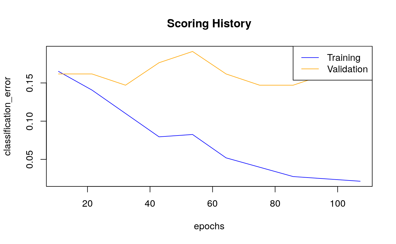
plot(dl_model,
     timestep = "samples",
     metric = "classification_error")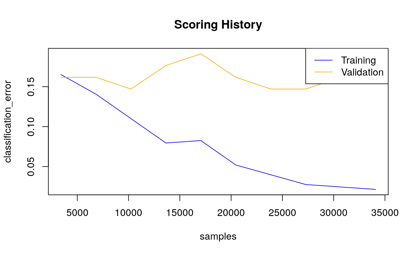
Next to the classification error, we are usually interested in the logistic loss (negative log-likelihood or log loss). It describes the sum of errors for each sample in the training or validation data or the negative logarithm of the likelihood of error for a given prediction/ classification. Simply put, the lower the loss, the better the model (if we ignore potential overfitting).
plot(dl_model,
     timestep = "epochs",
     metric = "logloss")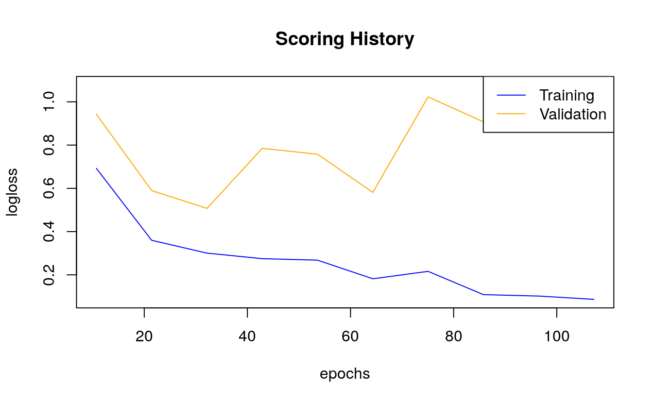
We can also plot the mean squared error (MSE). The MSE tells us the average of the prediction errors squared, i.e. the estimator’s variance and bias. The closer to zero, the better a model.
plot(dl_model,
     timestep = "epochs",
     metric = "rmse")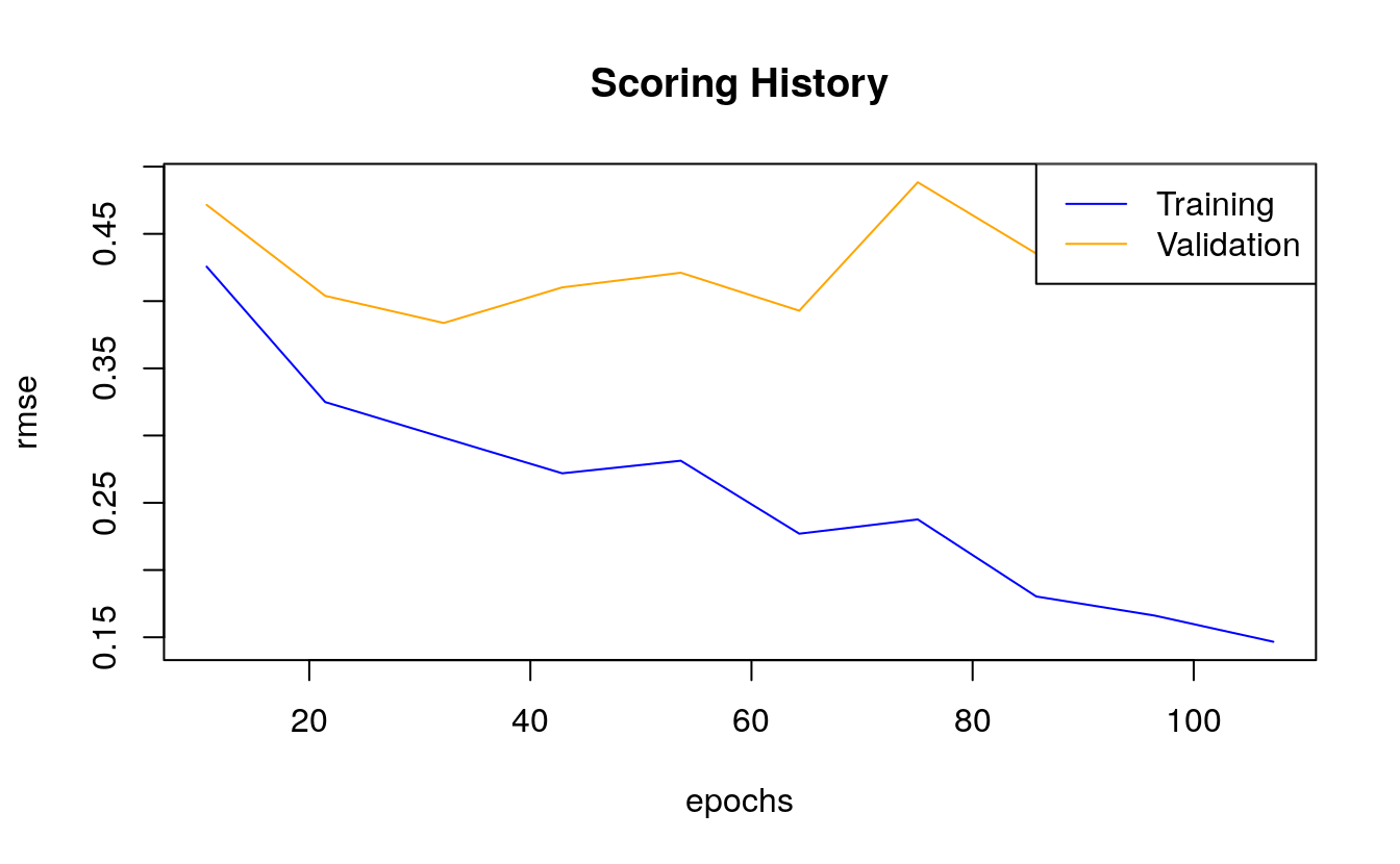
Next, we want to know the area under the curve (AUC). AUC is an important metric for measuring binary classification model performances. It gives the area under the curve, i.e. the integral, of true positive vs false positive rates. The closer to 1, the better a model.
h2o.auc(dl_model, train = TRUE)
#> [1] 0.994
h2o.auc(dl_model, valid = TRUE)
#> [1] 0.873
h2o.auc(dl_model, xval = TRUE)
#> [1] 0.836
The weights for connecting two adjacent layers and per-neuron biases that we specified the model to save, can be accessed with:
w <- h2o.weights(dl_model, matrix_id = 1)
b <- h2o.biases(dl_model, vector_id = 1)
Variable importance can be extracted as well (but keep in mind, that variable importance in deep neural networks is difficult to assess and should be considered only as rough estimates).
h2o.varimp(dl_model)
#> Variable Importances:
#>   variable relative_importance scaled_importance percentage
#> 1     V169            1.000000          1.000000   0.014803
#> 2       V5            0.920294          0.920294   0.013623
#> 3      V15            0.898893          0.898893   0.013306
#> 4       V7            0.876826          0.876826   0.012980
#> 5       V4            0.837585          0.837585   0.012399
#>
#> ---
#>    variable relative_importance scaled_importance percentage
#> 85     V168            0.672571          0.672571   0.009956
#> 86      V45            0.670279          0.670279   0.009922
#> 87     V249            0.668514          0.668514   0.009896
#> 88     V219            0.655353          0.655353   0.009701
#> 89      V33            0.650455          0.650455   0.009629
#> 90     V179            0.647482          0.647482   0.009585
h2o.varimp_plot(dl_model)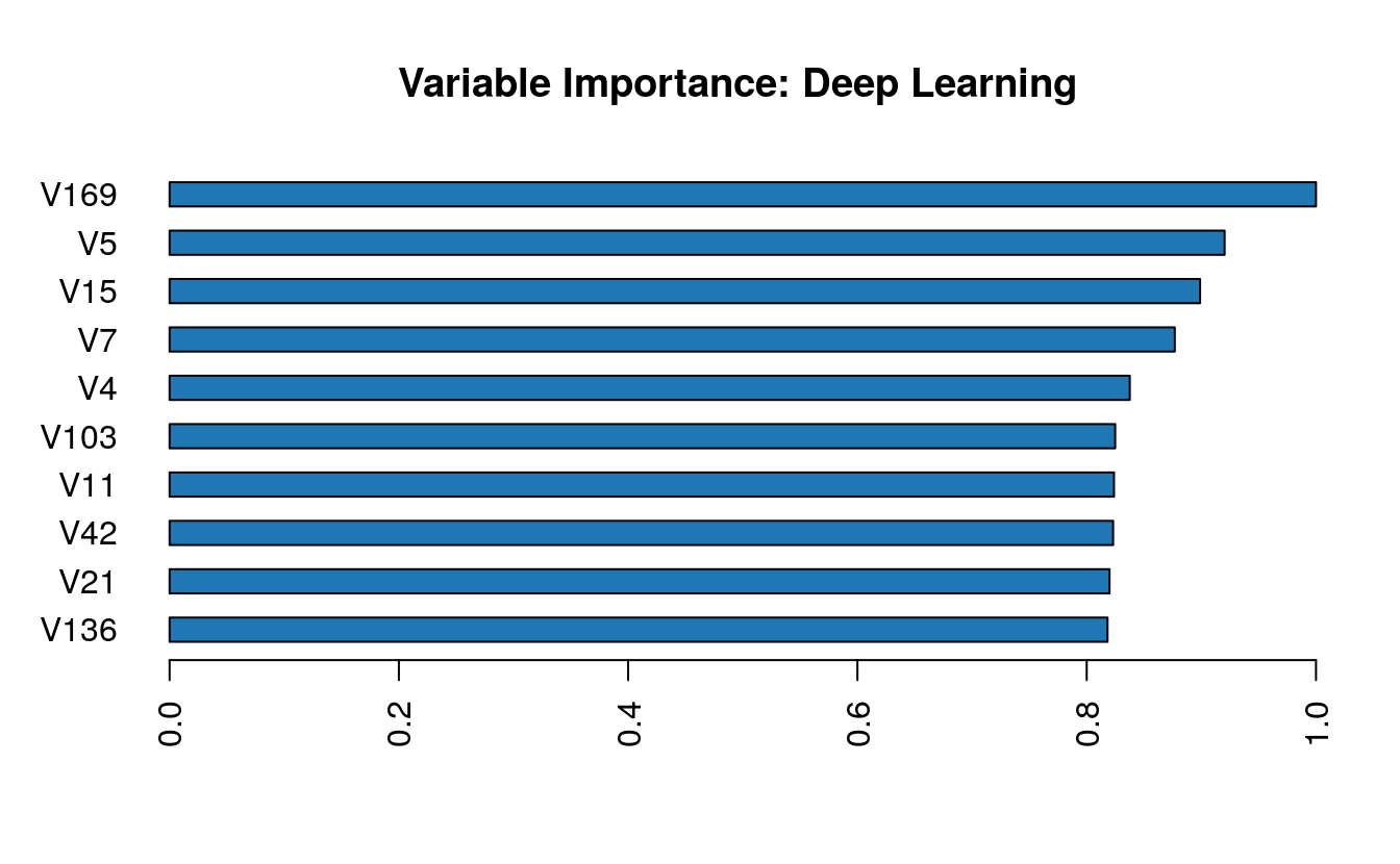
30.7 Test data
Now that we have a good idea about model performance on validation data, we want to know how it performed on unseen test data. A good model should find an optimal balance between accuracy on training and test data. A model that has 0% error on the training data but 40% error on the test data is in effect useless. It overfit on the training data and is thus not able to generalize to unknown data.
perf <- h2o.performance(dl_model, test)
perf
#> H2OBinomialMetrics: deeplearning
#>
#> MSE:  0.255
#> RMSE:  0.505
#> LogLoss:  1.88
#> Mean Per-Class Error:  0.315
#> AUC:  0.803
#> AUCPR:  0.826
#> Gini:  0.607
#>
#> Confusion Matrix (vertical: actual; across: predicted) for F1-optimal threshold:
#>            arrhythmia healthy    Error    Rate
#> arrhythmia         10      17 0.629630  =17/27
#> healthy             0      39 0.000000   =0/39
#> Totals             10      56 0.257576  =17/66
#>
#> Maximum Metrics: Maximum metrics at their respective thresholds
#>                         metric threshold     value idx
#> 1                       max f1  0.000001  0.821053  55
#> 2                       max f2  0.000001  0.919811  55
#> 3                 max f0point5  0.865327  0.828571  33
#> 4                 max accuracy  0.865327  0.772727  33
#> 5                max precision  0.998249  1.000000   0
#> 6                   max recall  0.000001  1.000000  55
#> 7              max specificity  0.998249  1.000000   0
#> 8             max absolute_mcc  0.865327  0.549349  33
#> 9   max min_per_class_accuracy  0.865327  0.743590  33
#> 10 max mean_per_class_accuracy  0.865327  0.779202  33
#> 11                     max tns  0.998249 27.000000   0
#> 12                     max fns  0.998249 38.000000   0
#> 13                     max fps  0.000000 27.000000  65
#> 14                     max tps  0.000001 39.000000  55
#> 15                     max tnr  0.998249  1.000000   0
#> 16                     max fnr  0.998249  0.974359   0
#> 17                     max fpr  0.000000  1.000000  65
#> 18                     max tpr  0.000001  1.000000  55
#>
#> Gains/Lift Table: Extract with `h2o.gainsLift(<model>, <data>)` or `h2o.gainsLift(<model>, valid=<T/F>, xval=<T/F>)`
Plotting the test performance’s AUC plot shows us approximately how good the predictions are.
plot(perf)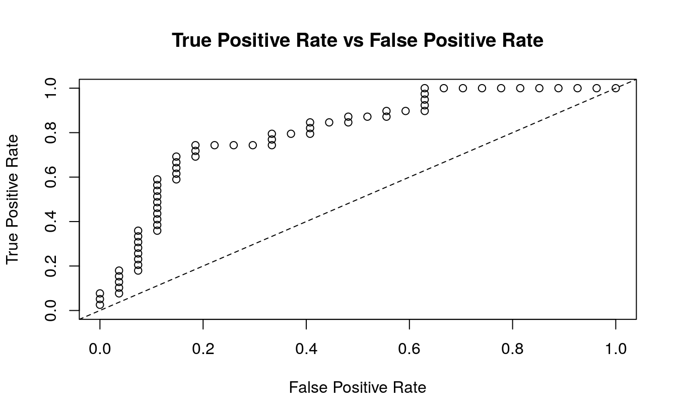 We also want to know the log loss, MSE and AUC values, as well as other model metrics for the test data:
h2o.logloss(perf)
#> [1] 1.88
h2o.mse(perf)
#> [1] 0.255
h2o.auc(perf)
#> [1] 0.803
head(h2o.metric(perf))
#> Metrics for Thresholds: Binomial metrics as a function of classification thresholds
#>   threshold       f1       f2 f0point5 accuracy precision   recall specificity
#> 1  0.998249 0.050000 0.031847 0.116279 0.424242  1.000000 0.025641    1.000000
#> 2  0.998113 0.097561 0.063291 0.212766 0.439394  1.000000 0.051282    1.000000
#> 3  0.998002 0.142857 0.094340 0.294118 0.454545  1.000000 0.076923    1.000000
#> 4  0.997845 0.139535 0.093750 0.272727 0.439394  0.750000 0.076923    0.962963
#> 5  0.997834 0.181818 0.124224 0.338983 0.454545  0.800000 0.102564    0.962963
#> 6  0.997818 0.222222 0.154321 0.396825 0.469697  0.833333 0.128205    0.962963
#>   absolute_mcc min_per_class_accuracy mean_per_class_accuracy tns fns fps tps
#> 1     0.103203               0.025641                0.512821  27  38   0   1
#> 2     0.147087               0.051282                0.525641  27  37   0   2
#> 3     0.181568               0.076923                0.538462  27  36   0   3
#> 4     0.082188               0.076923                0.519943  26  36   1   3
#> 5     0.121754               0.102564                0.532764  26  35   1   4
#> 6     0.155921               0.128205                0.545584  26  34   1   5
#>        tnr      fnr      fpr      tpr idx
#> 1 1.000000 0.974359 0.000000 0.025641   0
#> 2 1.000000 0.948718 0.000000 0.051282   1
#> 3 1.000000 0.923077 0.000000 0.076923   2
#> 4 0.962963 0.923077 0.037037 0.076923   3
#> 5 0.962963 0.897436 0.037037 0.102564   4
#> 6 0.962963 0.871795 0.037037 0.128205   5
The confusion matrix alone can be seen with the h2o.confusionMatrix() function, but is is also part of the performance summary.
h2o.confusionMatrix(dl_model, test)
#> Confusion Matrix (vertical: actual; across: predicted)  for max f1 @ threshold = 1.41603974479741e-06:
#>            arrhythmia healthy    Error    Rate
#> arrhythmia         10      17 0.629630  =17/27
#> healthy             0      39 0.000000   =0/39
#> Totals             10      56 0.257576  =17/66
The final predictions with probabilities can be extracted with the h2o.predict() function. Beware though, that the number of correct and wrong classifications can be slightly different from the confusion matrix above.
Here, I combine the predictions with the actual test diagnoses and classes into a data frame. For plotting I also want to have a column, that tells me whether the predictions were correct. By default, a prediction probability above 0.5 will get scored as a prediction for the respective category. I find it often makes sense to be more stringent with this, though and set a higher threshold. Therefore, I am creating another column with stringent predictions, where I only count predictions that were made with more than 80% probability. Everything that does not fall within this range gets scored as “uncertain”. For these stringent predictions, I am also creating a column that tells me whether they were accurate.
finalRf_predictions <- data.frame(class = as.vector(test$class),
                                  actual = as.vector(test$diagnosis),
                                  as.data.frame(h2o.predict(object = dl_model,
                                                            newdata = test)))
#>
  |
  |                                                                      |   0%
  |
  |======================================================================| 100%

finalRf_predictions$accurate <- ifelse(
  finalRf_predictions$actual == finalRf_predictions$predict, "yes", "no")

finalRf_predictions$predict_stringent <- ifelse(
  finalRf_predictions$arrhythmia > 0.8, "arrhythmia",
  ifelse(finalRf_predictions$healthy > 0.8, "healthy", "uncertain"))

finalRf_predictions$accurate_stringent <- ifelse(
  finalRf_predictions$actual == finalRf_predictions$predict_stringent, "yes",
  ifelse(finalRf_predictions$predict_stringent == "uncertain", "na", "no"))
finalRf_predictions %>%
  group_by(actual, predict) %>%
  summarise(n = n())
#> # A tibble: 4 x 3
#> # Groups:   actual [2]
#>   actual     predict        n
#>   <fct>      <fct>      <int>
#> 1 arrhythmia arrhythmia    13
#> 2 arrhythmia healthy       14
#> 3 healthy    arrhythmia     5
#> 4 healthy    healthy       34
finalRf_predictions %>%
  group_by(actual, predict_stringent) %>%
  summarise(n = n())
#> # A tibble: 6 x 3
#> # Groups:   actual [2]
#>   actual     predict_stringent     n
#>   <fct>      <chr>             <int>
#> 1 arrhythmia arrhythmia           18
#> 2 arrhythmia healthy               7
#> 3 arrhythmia uncertain             2
#> 4 healthy    arrhythmia            9
#> 5 healthy    healthy              29
#> 6 healthy    uncertain             1
To get a better overview, I am going to plot the predictions (default and stringent):
p1 <- finalRf_predictions %>%
  ggplot(aes(x = actual, fill = accurate)) +
    geom_bar(position = "dodge") +
    scale_fill_brewer(palette = "Set1") +
    my_theme() +
    labs(fill = "Were\npredictions\naccurate?",
         title = "Default predictions")

p2 <- finalRf_predictions %>%
  subset(accurate_stringent != "na") %>%
  ggplot(aes(x = actual, fill = accurate_stringent)) +
    geom_bar(position = "dodge") +
    scale_fill_brewer(palette = "Set1") +
    my_theme() +
    labs(fill = "Were\npredictions\naccurate?",
         title = "Stringent predictions")

grid.arrange(p1, p2, ncol = 2)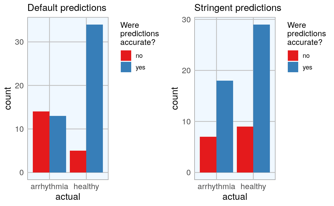
Being more stringent with the prediction threshold slightly reduced the number of errors but not by much.
I also want to know whether there are certain classes of arrhythmia that are especially prone to being misclassified:
p1 <- subset(finalRf_predictions, actual == "arrhythmia") %>%
  ggplot(aes(x = predict, fill = class)) +
    geom_bar(position = "dodge") +
    my_theme() +
    labs(title = "Prediction accuracy of arrhythmia cases",
         subtitle = "Default predictions",
         x = "predicted to be")

p2 <- subset(finalRf_predictions, actual == "arrhythmia") %>%
  ggplot(aes(x = predict_stringent, fill = class)) +
    geom_bar(position = "dodge") +
    my_theme() +
    labs(title = "Prediction accuracy of arrhythmia cases",
         subtitle = "Stringent predictions",
         x = "predicted to be")

grid.arrange(p1, p2, ncol = 2)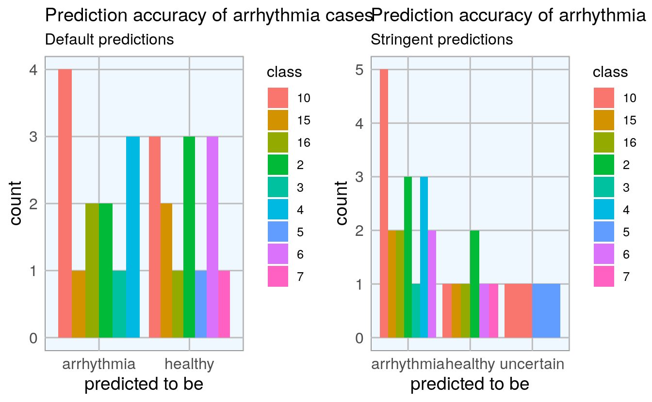
There are no obvious biases towards some classes but with the small number of samples for most classes, this is difficult to assess.
30.8 Final conclusions: How useful is the model?
Most samples were classified correctly, but the total error was not particularly good. Moreover, when evaluating the usefulness of a specific model, we need to keep in mind what we want to achieve with it and which questions we want to answer. If we wanted to deploy this model in a clinical setting, it should assist with diagnosing patients. So, we need to think about what the consequences of wrong classifications would be. Would it be better to optimize for high sensitivity, in this example as many arrhythmia cases as possible get detected - with the drawback that we probably also diagnose a few healthy people? Or do we want to maximize precision, meaning that we could be confident that a patient who got predicted to have arrhythmia does indeed have it, while accepting that a few arrhythmia cases would remain undiagnosed? When we consider stringent predictions, this model correctly classified 19 out of 27 arrhythmia cases, but 6 were misdiagnosed. This would mean that some patients who were actually sick, wouldn’t have gotten the correct treatment (if decided solely based on this model). For real-life application, this is obviously not sufficient!
Next week, I’ll be trying to improve the model by doing a grid search for hyper-parameter tuning.
So, stay tuned… (sorry, couldn’t resist ;-))
sessionInfo()
#> R version 3.6.3 (2020-02-29)
#> Platform: x86_64-pc-linux-gnu (64-bit)
#> Running under: Debian GNU/Linux 10 (buster)
#>
#> Matrix products: default
#> BLAS/LAPACK: /usr/lib/x86_64-linux-gnu/libopenblasp-r0.3.5.so
#>
#> locale:
#>  [1] LC_CTYPE=en_US.UTF-8       LC_NUMERIC=C
#>  [3] LC_TIME=en_US.UTF-8        LC_COLLATE=en_US.UTF-8
#>  [5] LC_MONETARY=en_US.UTF-8    LC_MESSAGES=C
#>  [7] LC_PAPER=en_US.UTF-8       LC_NAME=C
#>  [9] LC_ADDRESS=C               LC_TELEPHONE=C
#> [11] LC_MEASUREMENT=en_US.UTF-8 LC_IDENTIFICATION=C
#>
#> attached base packages:
#>  [1] stats4    parallel  grid      stats     graphics  grDevices utils
#>  [8] datasets  methods   base
#>
#> other attached packages:
#>  [1] reshape2_1.4.4       tidyr_1.0.2          matrixStats_0.56.0
#>  [4] pcaGoPromoter_1.30.0 Biostrings_2.54.0    XVector_0.26.0
#>  [7] IRanges_2.20.2       S4Vectors_0.24.4     BiocGenerics_0.32.0
#> [10] ellipse_0.4.1        gridExtra_2.3        ggrepel_0.8.2
#> [13] ggplot2_3.3.0        h2o_3.30.0.1         dplyr_0.8.5
#>
#> loaded via a namespace (and not attached):
#>  [1] Rcpp_1.0.4.6         utf8_1.1.4           assertthat_0.2.1
#>  [4] digest_0.6.25        plyr_1.8.6           R6_2.4.1
#>  [7] RSQLite_2.2.0        evaluate_0.14        pillar_1.4.3
#> [10] zlibbioc_1.32.0      rlang_0.4.5          data.table_1.12.8
#> [13] jquerylib_0.1.2      blob_1.2.1           rmarkdown_2.5.3
#> [16] labeling_0.3         stringr_1.4.0        RCurl_1.98-1.2
#> [19] bit_1.1-15.2         munsell_0.5.0        compiler_3.6.3
#> [22] xfun_0.19.4          pkgconfig_2.0.3      htmltools_0.5.0.9003
#> [25] downlit_0.2.1.9000   tidyselect_1.0.0     tibble_3.0.1
#> [28] bookdown_0.21.4      fansi_0.4.1          crayon_1.3.4
#> [31] withr_2.2.0          bitops_1.0-6         rappdirs_0.3.1
#> [34] jsonlite_1.6.1       gtable_0.3.0         lifecycle_0.2.0
#> [37] DBI_1.1.0            magrittr_1.5         scales_1.1.0
#> [40] cli_2.0.2            stringi_1.4.6        farver_2.0.3
#> [43] fs_1.4.1             xml2_1.3.2           bslib_0.2.2.9000
#> [46] ellipsis_0.3.0       vctrs_0.2.4          RColorBrewer_1.1-2
#> [49] tools_3.6.3          bit64_0.9-7          Biobase_2.46.0
#> [52] glue_1.4.0           purrr_0.3.4          yaml_2.2.1
#> [55] AnnotationDbi_1.48.0 colorspace_1.4-1     memoise_1.1.0
#> [58] knitr_1.28           sass_0.2.0.9005