18 Who buys Social Network ads
Datasets:
Social_Network_Ads.csv-
Algorithms:
- Support Vector Machines
18.2 Introduction
Source: https://www.geeksforgeeks.org/classifying-data-using-support-vector-machinessvms-in-r/
18.3 Data Operations
18.3.2 Importing the dataset
# Importing the dataset
dataset = read.csv(file.path(data_raw_dir, 'Social_Network_Ads.csv'))
dplyr::glimpse(dataset)
#> Rows: 400
#> Columns: 5
#> $ User.ID         <int> 15624510, 15810944, 15668575, 15603246, 15804002, 157…
#> $ Gender          <fct> Male, Male, Female, Female, Male, Male, Female, Femal…
#> $ Age             <int> 19, 35, 26, 27, 19, 27, 27, 32, 25, 35, 26, 26, 20, 3…
#> $ EstimatedSalary <int> 19000, 20000, 43000, 57000, 76000, 58000, 84000, 1500…
#> $ Purchased       <int> 0, 0, 0, 0, 0, 0, 0, 1, 0, 0, 0, 0, 0, 0, 0, 0, 1, 1,…
tibble::as_tibble(dataset)
#> # A tibble: 400 x 5
#>    User.ID Gender   Age EstimatedSalary Purchased
#>      <int> <fct>  <int>           <int>     <int>
#> 1 15624510 Male      19           19000         0
#> 2 15810944 Male      35           20000         0
#> 3 15668575 Female    26           43000         0
#> 4 15603246 Female    27           57000         0
#> 5 15804002 Male      19           76000         0
#> 6 15728773 Male      27           58000         0
#> # … with 394 more rows
# Taking columns 3-5
dataset = dataset[3:5]
tibble::as_tibble(dataset)
#> # A tibble: 400 x 3
#>     Age EstimatedSalary Purchased
#>   <int>           <int>     <int>
#> 1    19           19000         0
#> 2    35           20000         0
#> 3    26           43000         0
#> 4    27           57000         0
#> 5    19           76000         0
#> 6    27           58000         0
#> # … with 394 more rows
18.3.3 Encoding the target feature as factor
# Encoding the target feature as factor
dataset$Purchased = factor(dataset$Purchased, levels = c(0, 1))
str(dataset)
#> 'data.frame':    400 obs. of  3 variables:
#>  $ Age            : int  19 35 26 27 19 27 27 32 25 35 ...
#>  $ EstimatedSalary: int  19000 20000 43000 57000 76000 58000 84000 150000 33000 65000 ...
#>  $ Purchased      : Factor w/ 2 levels "0","1": 1 1 1 1 1 1 1 2 1 1 ...
18.3.4 Training and test datasets
# Splitting the dataset into the Training set and Test set
set.seed(123)
split = sample.split(dataset$Purchased, SplitRatio = 0.75)

training_set = subset(dataset, split == TRUE)
test_set = subset(dataset, split == FALSE) 18.3.6 Fitting SVM to the Training set
# Fitting SVM to the Training set
classifier = svm(formula = Purchased ~ .,
                 data = training_set,
                 type = 'C-classification',
                 kernel = 'linear')
classifier
#>
#> Call:
#> svm(formula = Purchased ~ ., data = training_set, type = "C-classification",
#>     kernel = "linear")
#>
#>
#> Parameters:
#>    SVM-Type:  C-classification
#>  SVM-Kernel:  linear
#>        cost:  1
#>
#> Number of Support Vectors:  116
summary(classifier)
#>
#> Call:
#> svm(formula = Purchased ~ ., data = training_set, type = "C-classification",
#>     kernel = "linear")
#>
#>
#> Parameters:
#>    SVM-Type:  C-classification
#>  SVM-Kernel:  linear
#>        cost:  1
#>
#> Number of Support Vectors:  116
#>
#>  ( 58 58 )
#>
#>
#> Number of Classes:  2
#>
#> Levels:
#>  0 1
18.3.7 Predicting the on the test dataset
# Predicting the Test set results
y_pred = predict(classifier, newdata = test_set[-3])
y_pred
#>   2   4   5   9  12  18  19  20  22  29  32  34  35  38  45  46  48  52  66  69
#>   0   0   0   0   0   0   0   0   0   0   0   0   0   0   0   0   0   0   0   0
#>  74  75  82  84  85  86  87  89 103 104 107 108 109 117 124 126 127 131 134 139
#>   0   0   0   0   0   0   0   0   0   1   0   0   0   0   0   0   0   0   0   0
#> 148 154 156 159 162 163 170 175 176 193 199 200 208 213 224 226 228 229 230 234
#>   0   0   0   0   0   0   0   0   0   0   0   0   1   1   1   0   1   0   1   1
#> 236 237 239 241 255 264 265 266 273 274 281 286 292 299 302 305 307 310 316 324
#>   1   0   1   1   1   0   1   1   1   1   1   0   1   1   1   0   1   0   0   0
#> 326 332 339 341 343 347 353 363 364 367 368 369 372 373 380 383 389 392 395 400
#>   0   1   0   1   0   1   1   0   1   1   1   0   1   0   1   1   0   0   0   0
#> Levels: 0 1
18.3.7.1 Confusion Matrix
# Making the Confusion Matrix
cm = table(test_set[, 3], y_pred)
cm
#>    y_pred
#>      0  1
#>   0 57  7
#>   1 13 23
xtable::xtable(cm)
#> % latex table generated in R 3.6.3 by xtable 1.8-4 package
#> % Fri Nov 20 00:16:35 2020
#> \begin{table}[ht]
#> \centering
#> \begin{tabular}{rrr}
#>   \hline
#>  & 0 & 1 \\
#>   \hline
#> 0 &  57 &   7 \\
#>   1 &  13 &  23 \\
#>    \hline
#> \end{tabular}
#> \end{table}
18.4 End
18.4.1 Plotting the training dataset
# installing library ElemStatLearn
# library(ElemStatLearn)

# Plotting the training data set results
set = training_set
X1 = seq(min(set[, 1]) - 1, max(set[, 1]) + 1, by = 0.01)
X2 = seq(min(set[, 2]) - 1, max(set[, 2]) + 1, by = 0.01)

grid_set = expand.grid(X1, X2)
colnames(grid_set) = c('Age', 'EstimatedSalary')
y_grid = predict(classifier, newdata = grid_set)

plot(set[, -3],
     main = 'SVM (Training set)',
     xlab = 'Age', ylab = 'Estimated Salary',
     xlim = range(X1), ylim = range(X2))

contour(X1, X2, matrix(as.numeric(y_grid), length(X1), length(X2)), add = TRUE)

points(grid_set, pch = '.', col = ifelse(y_grid == 1, 'coral1', 'aquamarine'))

points(set, pch = 21, bg = ifelse(set[, 3] == 1, 'green4', 'red3')) 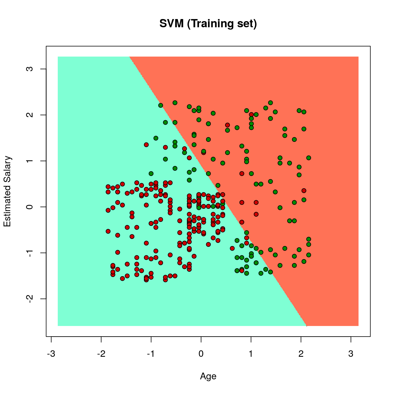
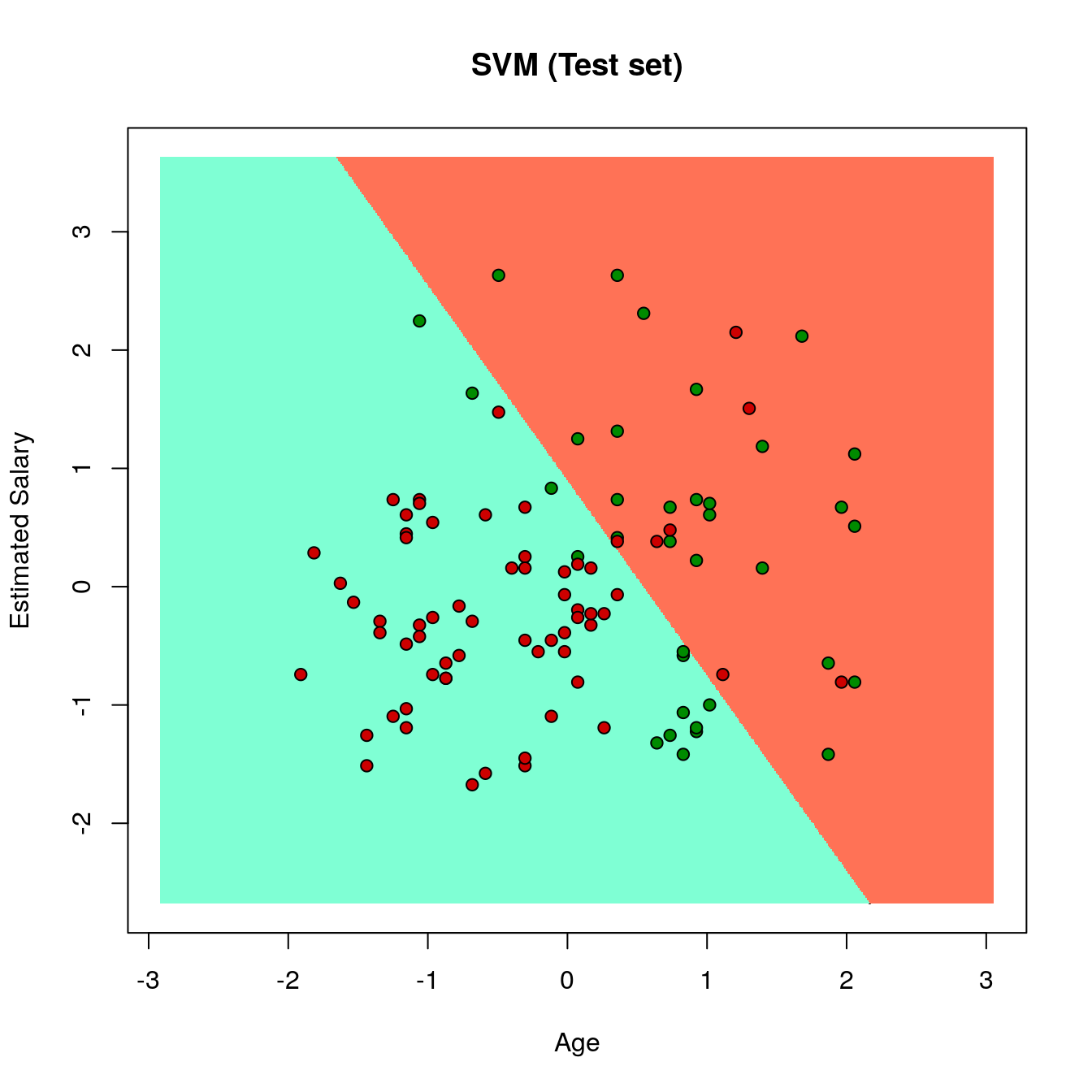
18.4.2 Plotting the test dataset
set = test_set
X1 = seq(min(set[, 1]) - 1, max(set[, 1]) + 1, by = 0.01)
X2 = seq(min(set[, 2]) - 1, max(set[, 2]) + 1, by = 0.01)

grid_set = expand.grid(X1, X2)
colnames(grid_set) = c('Age', 'EstimatedSalary')
y_grid = predict(classifier, newdata = grid_set)

plot(set[, -3], main = 'SVM (Test set)',
     xlab = 'Age', ylab = 'Estimated Salary',
     xlim = range(X1), ylim = range(X2))

contour(X1, X2, matrix(as.numeric(y_grid), length(X1), length(X2)), add = TRUE)

points(grid_set, pch = '.', col = ifelse(y_grid == 1, 'coral1', 'aquamarine'))

points(set, pch = 21, bg = ifelse(set[, 3] == 1, 'green4', 'red3'))